MATLAB: a tool of the future or an expensive toy. General information about MATLAB Matlab program overview
MatLab was created by Math Works over ten years ago. The work of hundreds of scientists and programmers is aimed at constantly expanding its capabilities and improving the underlying algorithms. Currently MatLab is a powerful and versatile tool for solving problems arising in various fields of human activity.
MatLab 6.x working environment, MatLab 7 has user-friendly interface to access many MatLab auxiliary elements.
When starting MatLab 6.x, the working environment appears on the screen ,
shown in Fig. one.
Rice. 1. Working environment of the MatLab 6.x package
This lesson teaches the basics of working (introduction) in matlab.
The working environment contains the following elements:
Menu;
- toolbar with buttons and a drop-down list;
- tabbed window Launch Pad and Workspace, from which you can get easy access to various ToolBox modules and to the contents of the working environment;
- tabbed window Command History and Current Directory, intended for viewing and recalling previously entered commands, as well as for setting the current directory;
- command window Command Window with the command line in which the blinking cursor is located;
- status bar.
All commands described in this lab should be typed at the command line. You do not need to type the "character itself" that denotes the command line prompt shown in the examples. It is convenient to use scroll bars or keys to view the work area.
It is important to remember that the typing of any command or expression must end with a key press
Remark 1
If some of the described windows are missing in the MatLab 6.x working environment, then go to the menu View select the appropriate items: Command Window, Command History, Current Directory, Workspace, Launch Pad.
2.1. Arithmetic calculations
MatLab's built-in math functions allow you to find the values of various expressions. MatLab provides the ability to control the output format of the result. Commands for evaluating expressions have a form common to all high-level programming languages.
2.1.1. The simplest calculations
Type 1 + 2 at the command line and press
»1 + 2
ans =
3
» |
What has MatLab done? First, she calculated the sum of 1 + 2, then wrote the result to the special variable ans and printed its value, equal to 3, to the command window. Below the answer is a command line with a blinking cursor, indicating that MatLab is ready for further calculations. You can type new expressions at the command line and find their values.
If you need to continue working with the previous expression, for example, calculate (1 + 2) /4.5, then the easiest way is to use the already existing result, which is stored in the ans variable. Type ans / 4.5 on the command line (decimal points are entered with a period) and press
»Ans / 4.5
ans =
0.6667
» |
Remark 2
The form in which the calculation results are displayed depends on the output format set in MatLab. The following explains how to set the basic output formats.
2.1.2. Calculation output formats
The required output format is defined by the user from the MatLab menu. Select from the menu File paragraph Preferences. A dialog box will appear on the screen. Preferences. To set the output format, make sure that the item is selected in the list of the left pane. Command Window... The format is set from the drop-down list Numeric format panels Text display.
So far, we will analyze only the most frequently used formats. Please select short in the dropdown Numeric format in MatLab 6.x. Close the dialog by clicking OK. The short floating-point format short is now used for displaying the results of calculations, in which only four digits after the decimal point are displayed on the screen. Type 100/3 at the command line and press
The result is output in short format:
"100/3
ans =
33.3333
This output format will be retained for all subsequent calculations, unless a different format is specified. Note that in MatLab a situation is possible when, when displaying a too large or small number, the result does not fit into the short format. Calculate 100000/3, the result is displayed in exponential form:
"100000/3
ans =
Z.ZZZZe + 004
The same will happen when finding 1/3000:
"1/3000
ans =
Z.ZZZZe-004
However, the original setting of the format is preserved and upon further calculations, for small numbers, the output will again be in short format.
In the previous example, the MatLab package displayed the result of calculations in exponential form. The entry 3.3333e-004 means 3.3333 * 10-4 or 0.00033333. Similarly, you can type numbers in expressions. For example, it is easier to type 10e9 or l.0e10 than 1,000,000,000, and the result will be the same. Space between digits and e is not allowed when entering, because this will produce an error message:
»10 e9
??? 10 е9
If you want to get the result of calculations more accurately, then you should select in the drop-down list long... The result will be displayed in long floating point format with fourteen digits after the decimal point. Formats short e and long e are designed to display the result in exponential form with four and fifteen digits after the decimal point, respectively. Information about formats can be obtained by typing the help command with the format argument at the command line:
A description of each format appears in the command window.
You can set the output format directly from the command line using the format command. For example, to set a long floating point format for the output of calculation results, enter the format long e command at the command line:
»Format long e
"1.25 / 3.11
ans =
4.019292604501608e-001
Note that the help format command displays the format names in capital letters. However, the command to be entered is in lowercase letters. This feature of the built-in help takes some getting used to. MatLab distinguishes between uppercase and lowercase letters. Attempting to type the command in capital letters will result in an error:
»FORMAT LONG E
??? FORMAT LONG.
Missing operator, comma, or semi-colon.
For a more convenient perception of the result, MatLab displays the result of calculations through a line after the calculated expression. However, sometimes it is convenient to place more lines on the screen by selecting the radio button compact (File, Numeric display) from the dropdown list. Adding blank lines is provided by choosing loose from the dropdown Numeric display.
Remark 3
All intermediate calculations are performed by MatLab with double precision, no matter what output format is set.
2.2. Using elementary functions
Suppose you want to evaluate the following expression:
Enter this expression in the command line according to MatLab rules and press
»Exp (-2.5) * log (11.3) ^ 0.3-sqrt ((sin (2.45 * pi) + cos (3.78 * pi)) / tan (3.3))
The answer is displayed in the command window:
ans =
-3.2105
When entering the expression, the built-in MatLab functions were used to calculate the exponent, natural logarithm, square root and trigonometric functions. What built-in atomic functions can I use and how can I call them? Type the command help eifun in the command line, and a list of all built-in elementary functions with their brief description is displayed in the command window. Function arguments are enclosed in parentheses, and function names are in lowercase. To enter a number l just type pi on the command line.
Arithmetic operations in MatLab are performed in the usual order typical of most programming languages:
Exponentiation ^;
- multiplication and division *, /;
- addition and subtraction +, -.
Use parentheses to change the order of execution of arithmetic operators.
If now you need to calculate the value of an expression similar to the previous one, for example
it is not necessary to type it again on the command line. You can use the fact that MatLab remembers all entered commands. To re-enter them into the command line, use the keys
1. Press the key<>, and the previously entered expression appears on the command line.
2. Make the necessary changes to it, replacing the minus sign with a plus and the square root for squaring (to move along the line with the expression, use the keys, , , ).
3. Evaluate the modified expression by pressing.
It turns out
»Exp (-2.5) * log (11.3) ^ 0.3 + ((sin (2.45 * pi) + cos (3.78 * pi)) / tan (3.3)) ^ 2
ans =
121.2446
If you need to get a more accurate result, then you should execute the command format long e, then press the key<>until the required expression appears on the command line, and evaluate it by pressing
»Format long e
»Exp (-2.5) * log (11.3) ^ 0.3 + ((sin. (2.45 * pi) + cos (3.78 * pi)) / tan (3.3)) ^ 2
ans =
1.212446016556763e + 002
You can display the result of the last found expression in a different format without recalculation. You should change the format with the short command, and then see the value of the ans variable by typing it in the command line and pressing
»Format short
»Ans
ans =
121.2446
In the MatLab 6.x working environment, there is a convenient tool for calling previously entered commands - a window Command History with command history. The command history contains the time and date of each MatLab 6.x session. To activate the window Command History you must select the tab with the same name. The current command in the window is shown with a blue background. If you click on any command in the window with the left mouse button, then this command becomes the current one. To execute it in MatLab, you need to double-click or select a line with a command using the keys
When right clicking on the window area Command History a pop-up menu appears. Item selection Soru causes the command to be copied to the Windows clipboard. With help Evaluate Selection you can execute the marked group of commands. To delete the current command, use the item Delete Selection. D To remove all commands up to the current one - Delete to Selection, to remove all commands - Delete Entire History.
During calculations, some exceptional situations are possible, for example division by zero, which in most programming languages lead to an error. When dividing a positive number by zero in MatLab, inf (infinity) is obtained, and when dividing negative number zero is -inf (minus infinity) and a warning is issued:
»1/0
Warning: Divide by zero.
ans =
Inf
Dividing zero by zero results in NaN (not a number) and also generates a warning:
»
0/0
Warning: Divide by zero.
ans =
NaN
When calculating like sqrt (-1) , no error or warning is raised. MatLab automatically goes into the complex numbers area:
»Sqrt (-1.0)
ans =
0 + l.0000i
How do I know which built-in atomic functions can be used and how to call them? Type the command at the command prompt help eifun, at the same time a list of all built-in elementary functions with their brief description is displayed in the command window.
MATLAB combines an easy-to-learn language with a fast computation speed. What makes this performance so fast? What do you need to do to write a really fast program in MATLAB? Finally, is there a decent free software alternative to MATLAB? We will try to answer all these questions now.
MATLAB emerged in the late 1970s as a scripting language and wrapper around the LINPACK and EISPACK linear algebra library functions. A feature of MATLAB is that the base (and at that time - the only) data type in it is a matrix, not a number. Thanks to this, it was possible to save the writing of matrix operations from cycles, making it more compact and similar to mathematical. On the other hand, the use of the most modern libraries at that time ensured high speed of calculations. All of this has contributed to the rapid rise in popularity of MATLAB.
Multiplying a matrix by a number written in different ways
More than thirty years have passed since then. Over the years, dozens of books have been written about MATLAB; it has become one of the standard languages for scientific and technical calculations. The relative simplicity of the language and the high speed of computations performed with it have been preserved and still remain the attractive aspects of the package. But how is this achieved? How does modern MATLAB work?
As before, MATLAB has the most advanced math libraries under the hood. Now these are: Intel Math Kernel Library (MKL) for linear algebra operations and Intel Integrated Performance Primitives Library (IPPL) for optimizing image processing. MKL includes, in particular, libraries: BLAS, which implements basic vector-matrix operations, and LAPACK, a modern development of LINPACK, containing linear algebra problem solvers. Therefore, it is not surprising that MATLAB outperforms any "home-made" code that implements vector-matrix operations in terms of execution speed. It also confidently bypasses packages that use other BLAS and LAPACK implementations.
The fact is that MKL and IPPL use SSE and AVX - sets of instructions for the processor that implement parallel computations, in the case when you need to perform the same sequence of actions on different data (SIMD). This leads to a significant increase in productivity, and without any effort on the part of the user.
In addition, MATLAB probably uses SSE / AVX in its kernel functions, which are implemented in C. At least for the development of the MathWorks package, it uses Intel Parallel Studio XE, which includes a C / C ++ compiler.
Curiously, on computers with AMD processors, MATLAB also uses libraries developed by Intel, although AMD has implemented its own library with similar capabilities - AMD Core Math Library (ACML).
Thus, MATLAB performance is made up of highly optimized libraries (Intel), implicit parallelization (which is also a credit to Intel) and kernel functions tuned to take advantage of these advantages (MathWorks). We cannot know the exact degree of influence of each of the factors, in addition, they can vary from version to version and from platform to platform.

Determining the Versions of the Libraries Used by MATLAB Using the Version Function
In order to effectively use these capabilities, it is necessary to "vectorize" the program, that is, to replace the use of loops with operations on the array as a whole, which are exactly implemented by fast MATLAB functions.
But the cycles were not forgotten either. In 2003, a JIT compiler appeared as part of MATLAB (version 6.5, R13). It analyzes the program being executed by translating repetitive fragments into machine code. As a result, with subsequent repetitions, the execution speed of these fragments increases significantly (sometimes up to 100 times), which makes some loops almost as fast as their vectorized counterparts. But: in order for the JIT compiler to be successfully applied, the loop code must meet certain requirements.
A brief summary of these requirements, as well as tips for vectorizing the program, can be found in the Writing Fast MATLAB Code, and for more detailed and up-to-date information - in Yair Altman's Undocumented Matlab blog or on the pages of his book “Accelerating MATLAB Performance” - the most detailed one to date See the MATLAB Program Optimization Guide. By the way, the above use of the version function also applies to the undocumented features of the package.
As a cheaper alternative to MATLAB, you can use Python with the NumPy / SciPy libraries and MKL installed. In this case, instead of the MATLAB JIT compiler, Numba or Cython are used. Numerous tests, the results of which can be found on the Internet (for example, this one), indicate that MATLAB and the Python + SciPy bundle produce very similar results in terms of speed, so the programmer's skill and knowledge of the features of a particular package come to the fore.
Dmitry Khramov
Those who deal with higher mathematics know very well what kind of mathematical "monsters" you sometimes have to face. For example, calculating some giant triple integral can take a lot of time, mental strength and non-regenerating nerve cells. Of course, it's very interesting to challenge the integral and take it. But what if the integral threatens to take you instead? Or worse, did the cubic trinomial get out of control and rage? You wouldn't wish that on an enemy either.

Previously, there were only two options: to spit on everything and go for a walk, or to engage in a multi-hour battle with the integral. Well, to whom many hours, to whom many minutes - who studied how. But that's not the point. The twentieth century and the inexorably moving progress offer us a third way, namely, they allow us to take the most complex integral "in a quick way". The same goes for solving all kinds of equations, plotting functions in the form of cubic hyperboloids, etc.
For such extraordinary, but periodically occurring situations among students, there is a powerful mathematical weapon. Meet those who don't know yet - the MATLAB software package.
Matlab will both solve the equation, and approximate, and plot the function. Do you understand what this means, friends?
This means that it is one of the most powerful data processing packages available today. The name stands for MatrixLaboratory. Matrix Laboratory, if in russian . The capabilities of the program cover almost all areas of mathematics. So, using matlab, you can:
- Perform all kinds of operations on matrices, solve linear equations, work with vectors;
- Calculate the roots of polynomials of any degree, perform operations on polynomials, differentiate, extrapolate and interpolate curves, build graphs of any functions;
- Conduct statistical analysis data using digital filtering, statistical regression;
- Solve differential equations. In partial derivatives, linear, nonlinear, with boundary conditions - it doesn't matter, matlab will solve everything;
- Perform integer arithmetic operations.

In addition to all this, MATLAB's capabilities allow you to visualize data up to the construction of three-dimensional graphs and the creation of animated videos.
Our description of matlab, of course, is far from complete. In addition to the features and functions provided by the manufacturer, there is great amount Matlab tools written by enthusiasts or other companies.
MATLAB as a programming language

It is also a programming language used directly when working with the program. We will not go into details, let's just say that programs written in MATLAB are of two types: functions and scripts.

The main working file of the program is the M-file. This is an endless text file, and it is in it that the actual programming of calculations takes place. By the way, don't be intimidated by this word - you don't need to be a professional programmer to work in MATLAB.
M-files are divided into
- M-scripts. An M script is the simplest type of M file and has no input and output arguments. This file used to automate repetitive calculations.
- M-functions. M-functions are M-files that allow input and output arguments.
In order to clearly show how work is done in MATLAB, we give an example of creating a function in matlab below. This function will calculate the average of the vector.
f
unction y = average (x)
% AVERAGE Average value of vector elements.
% AVERAGE (X), where X is a vector. Calculates the average of the elements in a vector.
% If the input argument is not a vector, an error is generated.
= size (x);
if (~ ((m == 1) | (n == 1)) | (m == 1 & n == 1))
error ("The input array must be a vector")
end
y = sum (x) / length (x); % The actual calculation
The function definition line tells the MATLAB system that the file is an M-function and also defines a list of input arguments. So, the definition line of the average function looks like this:
function y = average (x)
Where:
- function is a keyword defining an M-function;
- y is the output argument;
- average - function name;
- x is an input argument.
So, to write a function in matlab, you need to remember that every function in MATLAB contains a function definition line like the one below.
Of course, such a powerful package is needed not only to make life easier for students. Nowadays MATLAB, on the one hand, is very popular among specialists in many scientific and engineering fields. On the other hand, the ability to work with large matrices makes MATLAB an indispensable tool for financial analysts, allowing you to solve many more problems than, for example, the well-known Excel. You can read more about that in the review article.
Disadvantages of working with MATLAB

What are the difficulties in working with MATLAB? There is perhaps only one difficulty. But fundamental. In order to fully reveal the capabilities of MATLAB and easily solve the problems facing you, you will have to sweat and first deal with the matlab itself (how to create a file, how to create a function, etc.). And this is not so easy, because the power and ample opportunities require sacrifices.
With all the desire, one cannot say that MATLAB is -simple program. Nevertheless, we hope that all of the above will be sufficient reason to start mastering it.
And finally. If you do not know why everything in your life has gone this way and not otherwise, ask the matlab about it. Just type “why” at the command line. He will answer. Try it!
Now you know the possibilities of Matlab. In education, MATLAB is often used in teaching numerical methods and linear algebra. Many students cannot do without it when processing the results of an experiment carried out in the course of laboratory work. For quick and high-quality mastering of the basics of working with MATLAB, you can always turn to, at any time ready to answer any of your questions.
1. Lesson 23. Introducing MATLAB Extension Packs
Lesson number 23.
Acquaintance with MATLAV expansion packs
List Expansion Packages
Simulinc for Windows
Symbolic Mathematics Package
Math packages
Analysis and synthesis packages for control systems
System identification packages
Additional Simulinc Tools
Signal and Image Processing Packages
Other application packages
In this lesson, we will briefly familiarize ourselves with the basic means of professional expansion of the system and its adaptation for solving certain classes of mathematical and scientific and technical problems - with the MATLAB system extension packages. There is no doubt that at least a part of these packages should be devoted to a separate training course or reference book, perhaps more than one. Separate books have been published for most of these extensions abroad, and the volume of documentation on them amounts to hundreds of megabytes. Unfortunately, the length of this book only allows you to walk a little through the expansion packs in order to give the reader an idea of where the system is headed.
2. Listing expansion packs
List Expansion Packages
The complete MATLAB 6.0 system contains a number of components, the name, version number and creation date of which can be displayed with the ver command:
MATLAB Version 6.0.0.88 (R12) on PCWIN MATLAB License Number: 0
|
MATLAB Toolbox |
Version 6.0 |
06-0ct-2000 |
|||
|
Version 4.0 |
|||||
|
Version 4.0 |
04-0ct-2000 |
||||
|
Stateflow coder |
Version 4.0 |
04-0ct-2000 |
|||
|
Real -Time Workshop |
Version 4.0 |
||||
|
COMA Reference Blockset |
Version 1.0.2 |
||||
|
Communications blockset |
Version 2.0 |
||||
|
Communications Toolbox |
Version 2.0 |
||||
|
Control System Toolbox |
Version 5.0 |
||||
|
DSP Blockset |
Version 4.0 |
||||
|
Data Acquisition Toolbox |
Version 2.0 |
05-0ct-2000 |
|||
|
Database Toolbox |
Version 2.1 |
||||
|
Datafeed Toolbox |
Version 1.2 |
||||
|
Dials & gauges blockset |
Version 1.1 |
||||
|
Filter Design Toolbox |
Version 2.0 |
||||
|
Financial Derivatives Toolbox |
Version 1.0 |
||||
|
Financial Time Series Toolbox |
Version 1.0 |
||||
|
Financial Toolbox |
Version 2.1.2 |
||||
|
Fixed-Point Blockset |
Version 3.0 |
||||
|
Fuzzy Logic Toolbox |
Version 2.1 |
||||
|
GARCH Toolbox |
Version 1.0 |
||||
|
Image Processing Toolbox |
Version 2.2.2 |
|
Instrument Control Toolbox |
Version 1.0 |
||||
|
LMI Control Toolbox |
Version 1.0.6 |
||||
|
MATLAB Compiler |
Version 2.1 |
||||
|
MATLAB Report Generator |
Version 1.1 |
||||
|
Mapping Toolbox |
Version 1.2 |
||||
|
|
Version 1.0.5 |
||||
|
Motorola DSP Developer "s Kit |
Version 1.1 |
Ol-Sep-2000 |
|||
|
Mi-Analysis and Synthesis Toolbox |
Version 3.0.5 |
||||
|
Neural Network Toolbox |
Version 4.0 |
||||
|
Nonlinear Control Design Blockset |
Version 1.1.4 |
||||
|
Optimization Toolbox |
Version 2.1 |
||||
|
Partial Differential Equation Toolbox |
Version 1.0.3 |
||||
|
Power System Blockset |
Version 2.1 |
||||
|
Real-Time Workshop Ada Coder |
Version 4.0 |
||||
|
Real-Time Workshop Embedded Coder |
Version 1.0 |
||||
|
Requirements Management Interface |
Version 1.0.1 |
||||
|
Robust control toolbox |
Version 2.0.7 |
||||
|
SB2SL (converts SystemBuild to Simu |
Version 2.1 |
||||
|
Signal Processing Toolbox |
Version 5.0 |
||||
|
Simulink Accelerator |
Version 1.0 |
||||
|
Model Differencing for Simulink and ... |
Version 1.0 |
||||
|
Simulink Model Coverage Tool |
Version 1.0 |
||||
|
Simulink Report Generator |
Version 1.1 |
||||
|
Spline Toolbox |
Version 3.0 |
||||
|
Statistics Toolbox |
Version 3.0 |
||||
|
Symbolic Math Toolbox |
Version 2.1.2 |
||||
|
|
Version 5.0 |
||||
|
Wavelet Toolbox |
Version 2.0 |
||||
|
Version 1.1 |
|||||
|
xPC Target Embedded Option |
Version 1.1 |
Please note that almost all expansion packs in MATLAB 6.0 have been updated and date back to 2000. Their description has been significantly expanded, which in PDF format already occupies many more than ten thousand pages. Below is a brief description of the main expansion packs
3. Simulink for Windows
Simulink for Windows
The Simulink extension package is used to simulate models consisting of graphic blocks with specified properties (parameters). Model components, in turn, are graphic blocks and models that are contained in a number of libraries and with the help of the mouse can be transferred to the main window and connected to each other by the necessary links. The models can include various types of signal sources, virtual recording devices, graphic animation tools. Double-clicking on the model block displays a window with a list of its parameters, which the user can change. The simulation launch provides mathematical modeling of the constructed model with a clear visual presentation of the results. The package is based on the construction of block diagrams by transferring blocks from the library of components to the editing window of a user-created model. Then the model is run. In fig. Figure 23.1 shows the process of modeling a simple system - a hydraulic cylinder. The control is carried out using virtual oscilloscopes - in Fig. Figure 23.1 shows the screens of two such oscilloscopes and the window of a simple subsystem of the model. It is possible to simulate complex systems consisting of many subsystems.
Simulink creates and solves the equations of state of the model and allows you to connect a variety of virtual measuring instruments to the desired points. The clarity of the presentation of the simulation results is striking. A number of examples of using the Simulink package have already been given in Lesson 4. The previous version of the package is described in sufficient detail in books. The main innovation is matrix signal processing. Added separate Simulink performance packages such as Simulink Accelerator for compiling model code, Simulink profiler for code analysis, etc.

Rice. 23.1. Example of Simulating a Hydraulic Cylinder System Using the Simulink Extension
1.gif
Image:
1b.gif
Image:
4. Real Time Windows Target and Workshop
Real Time Windows Target and Workshop
A powerful real-time simulation subsystem that connects to Simulink (with additional hardware in the form of computer expansion cards), represented by the Real Time Windows Target and Workshop expansion packs, is a powerful tool for managing real objects and systems. In addition, these extensions allow you to create executable model codes. Rice. 4.21 in lesson 4 shows an example of such modeling for a system described by nonlinear differential equations of van der Pol. The advantage of such modeling is its mathematical and physical clarity. In the components of Simulink models, you can specify not only fixed parameters, but also mathematical relationships that describe the behavior of the models.
5. Report Generator for MATLAB and Simulink
Report Generator for MATLAB and Simulink
Report Generators, a tool introduced in MATLAB 5.3.1, provides information about the operation of the MATLAB system and the Simulink add-on package. This tool is very useful when debugging complex computational algorithms or when simulating complex systems. Report generators are launched by the Report command. Reports can be presented in the form of programs and edited.
Report generators can run commands and program snippets included in reports and allow you to monitor the behavior of complex calculations.
6. Neural Networks Toolbox
Neural Networks Toolbox
A package of applied programs containing tools for constructing neural networks based on the behavior of a mathematical analogue of a neuron. The package provides effective support for the design, training and modeling of many known network paradigms, from basic perceptron models to the most advanced associative and self-organizing networks. The package can be used to research and apply neural networks to tasks such as signal processing, nonlinear control, and financial modeling. Provided the ability to generate portable C-code using Real Time Workshop.
The package includes more than 15 known types of networks and training rules that allow the user to choose the most suitable paradigm for a specific application or research problem. For each type of architecture and training rules, there are functions for initializing, training, adapting, creating and modeling, demonstrating, and a sample network application.
For managed networks, you can choose a forward or recurrent architecture using a variety of teaching rules and design techniques such as perceptron, backpropagation, Levenberg backpropagation, radial-based networks, and recurrent networks. You can easily change any architectures, teaching rules or transitional functions, add new ones - and all this without writing a single line in C or Fortran. An example of using the package for recognizing the pattern of a letter was given in lesson 4. A detailed description of the previous version of the package can be found in the book.
7. Fuzzy Logic Toolbox
Fuzzy Logic Toolbox
The Fuzzy Logic software package belongs to the theory of fuzzy (fuzzy) sets. Support is provided for modern methods of fuzzy clustering and adaptive fuzzy neural networks. The graphical tools of the package allow you to interactively monitor the peculiarities of the system's behavior.
Key features of the package:
- definition of variables, fuzzy rules and membership functions;
- interactive viewing of fuzzy inference;
- modern methods: adaptive fuzzy inference using neural networks, fuzzy clustering;
- interactive dynamic modeling in Simulink;
generating portable C code using Real-Time Workshop.
This example clearly shows the differences in the behavior of the model with and without fuzzy logic.
8. Symbolic Math Toolbox
Symbolic Math Toolbox
A package of applied programs that give the MATLAB system fundamentally new opportunities - the ability to solve problems in a symbolic (analytical) form, including the implementation of exact arithmetic of arbitrary bit width. The package is based on the use of the core of symbolic mathematics of one of the most powerful computer algebra systems - Maple V R4. Provides symbolic differentiation and integration, calculation of sums and products, expansion into Taylor and Maclaurin series, operations with power polynomials (polynomials), calculation of polynomial roots, solution of nonlinear equations in analytical form, all kinds of symbolic transformations, substitutions, and much more. Has commands for direct access to the Maple V system core.
The package allows you to prepare procedures with the syntax of the Maple V R4 programming language and install them in the MATLAB system. Unfortunately, in terms of the capabilities of symbolic mathematics, the package is much inferior to specialized computer algebra systems, such as the latest versions of Maple and Mathematica.
9. Packages of mathematical calculations
Math packages
MATLAB includes many add-on packages that enhance the mathematical capabilities of the system to improve the speed, efficiency, and accuracy of calculations.
10. NAG Foundation Toolbox
NAG Foundation Toolbox
One of the most powerful libraries mathematical functions created by the special group The Numerical Algorithms Group, Ltd. The package contains hundreds of new features. The names of the functions and the syntax for calling them are borrowed from the well-known NAG Foundation Library. As a result, experienced NAG FORTRAN users can easily work with the NAG package in MATLAB. The NAG Foundation library provides its functions in the form of object codes and corresponding m-files to call them. The user can easily modify these MEX files at the source level.
The package provides the following features:
roots of polynomials and the modified Laguerre method;
calculation of the sum of a series: discrete and Hermitian-discrete Fourier transform;
ordinary differential equations: Adams and Runge-Kutta methods;
partial differential equations;
interpolation;
calculation of eigenvalues and vectors, singular numbers, support for complex and real matrices;
approximation of curves and surfaces: polynomials, cubic splines, Chebyshev polynomials;
minimization and maximization of functions: linear and quadratic programming, extrema of functions of several variables;
decomposition of matrices;
solution of systems of linear equations;
linear equations (LAPACK);
statistical calculations, including descriptive statistics and probability distributions;
correlation and regression analysis: linear, multivariate and generalized linear models;
multidimensional methods: principal components, orthogonal rotation;
generation of random numbers: normal distribution, Poisson, Weibull and Koschi distributions;
nonparametric statistics: Friedman, Kruskal-Wallis, Mann-Whitney; Time series: one-dimensional and multidimensional;
approximation of special functions: integral exponent, gamma function, Bessel and Hankel functions.
Finally, this package allows the user to create FORTRAN programs that dynamically link with MATLAB.
11. Spline Toolbox
Application package for working with splines. Supports one-dimensional, two-dimensional and multidimensional spline interpolation and approximation. Provides presentation and display of complex data and graphics support.
The package allows you to perform interpolation, approximation and transformation of splines from B-form to piecewise polynomial, interpolation with cubic splines and smoothing, performing operations on splines: calculating the derivative, integral and display.
Spline is equipped with B-spline programs described in A Practical Guide to Splines by Carl Debour, spline creator and author of Spline. Package functions in conjunction with MATLAB language and detailed guidance make it easier for the user to understand splines and apply them effectively to solving a variety of problems.
The package includes programs for working with the two most widespread forms of spline representation: B-form and piecewise-polynomial form. The B-shape is useful during the spline construction phase, while the piecewise polynomial shape is more efficient during continuous spline work. The package includes functions for creating, displaying, interpolating, approximating and processing splines in B-form and in the form of polynomial segments.
12. Statistics Toolbox
Statistics Toolbox
A package of applied programs for statistics, dramatically expanding the capabilities of the MATLAB system in the implementation of statistical calculations and statistical data processing. Contains a very representative set of tools for generating random numbers, vectors, matrices and arrays with different distribution laws, as well as many statistical functions. It should be noted that the most common statistical functions are included in the core of the MATLAB system (including functions for generating random data with uniform and normal distribution). Key features of the package:
descriptive statistics;
probability distributions;
parameter estimation and approximation;
hypothesis testing;
multiple regression;
interactive stepwise regression;
Monte Carlo simulation;
interval approximation;
statistical process control;
planning an experiment;
response surface modeling;
approximation of a nonlinear model;
principal component analysis;
statistical graphs;
graphical user interface.
The package includes 20 different probability distributions, including t (Student), F, and Chi-square. Selection of parameters, graphical display of distributions and a method for calculating the best approximations are provided for all types of distributions. There are many interactive tools for dynamic data visualization and analysis. There are specialized interfaces for modeling response surfaces, visualizing distributions, generating random numbers and level lines.
13. Optimization Toolbox
Optimization Toolbox
Application package - for solving optimization problems and systems of nonlinear equations. Supports basic optimization methods for functions of a number of variables:
unconditional optimization of nonlinear functions;
least squares and nonlinear interpolation;
solving nonlinear equations;
linear programming;
quadratic programming;
conditional minimization of nonlinear functions;
minimax method;
multiobjective optimization.
A variety of examples demonstrate the effective use of the package functions. They can also be used to compare how the same problem is solved by different methods.
14. Partial Differential Equations Toolbox
Partial Differential Equations Toolbox
A very important application package containing many functions for solving systems of partial differential equations. Provides effective tools for solving such systems of equations, including stiff ones. The package uses a finite element method. The commands and the graphical interface of the package can be used for mathematical modeling of partial differential equations as applied to a wide class of engineering and scientific applications, including problems of resistance of materials, calculations of electromagnetic devices, problems of heat and mass transfer and diffusion. Key features of the package:
full-fledged graphical interface for processing second-order partial differential equations;
automatic and adaptive mesh selection;
setting boundary conditions: Dirichlet, Neumann and mixed;
flexible problem setting using MATLAB syntax;
fully automatic mesh partitioning and selection of the size of finite elements;
nonlinear and adaptive design schemes;
the ability to visualize the fields of various parameters and functions of the solution, a demonstration of the adopted partitioning and animation effects.
The package intuitively follows the six steps of solving a PDE using the finite element method. These steps and the corresponding modes of the package are as follows: determining the geometry (drawing mode), setting boundary conditions (boundary conditions mode), choosing the coefficients that define the problem (PDE mode), discretizing finite elements (mesh mode), setting initial conditions and solving equations (solution mode), post-processing of the solution (graph mode).
15. Packages of analysis and synthesis of control systems
Analysis and synthesis packages for control systems
Control System Toolbox
The Control System package is intended for modeling, analysis and design of automatic control systems - both continuous and discrete. The package functions implement traditional transfer function methods and modern state space methods. Frequency and time responses, zeros and poles diagrams can be quickly calculated and displayed on the screen. The package contains:
a complete set of tools for analyzing MIMO systems (many inputs - many outputs) systems;
time characteristics: transfer and transient functions, response to an arbitrary action;
frequency characteristics: Bode, Nichols, Nyquist diagrams, etc .;
development of feedbacks;
design of LQR / LQE-regulators;
characteristics of models: controllability, observability, lowering the order of models;
lagged systems support.
Additional model building functions allow you to construct more complex models. The time response can be calculated for a pulse input, a single hop, or an arbitrary input. There are also functions for analyzing singular numbers.
An interactive environment for comparing time and frequency responses of systems provides the user with graphical controls for simultaneously displaying and switching between responses. Various response characteristics such as acceleration and control times can be calculated.
The Control System package contains tools for selecting feedback parameters. Traditional methods include feature point analysis, gain and attenuation determination. Among modern methods: linear-quadratic regulation, etc. The Control System package includes a large number of algorithms for the design and analysis of control systems. In addition, it has a customizable environment and allows you to create your own m-files.
16. Nonlinear Control Design Toolbox
Nonlinear Control Design Toolbox
Nonlinear Control Design (NCD) Blockset implements a dynamic optimization method for the design of control systems. Designed for use with Simulink, this tool automatically adjusts system parameters based on user-defined timing constraints.
The package uses mouse transfer to change time constraints directly on graphs, which makes it easy to configure variables and specify undefined parameters, provides interactive optimization, implements Monte Carlo simulations, supports the design of SISO (one input - one output) and MIMO control systems , allows you to simulate interference cancellation, tracking and other types of responses, supports repeating parameter problems and control tasks with lagging systems, allows you to choose between satisfied and unattainable constraints.
17. Robust Control Toolbox
Robust control toolbox
The Robust Control package includes tools for the design and analysis of multi-parameter robust control systems. These are systems with simulation errors, the dynamics of which is not fully known or whose parameters may change during the simulation. Powerful algorithms of the package allow you to perform complex calculations taking into account changes in many parameters. Package features:
synthesis of LQG-controllers based on minimization of uniform and integral norms;
multi-parameter frequency response;
building a state space model;
transformation of models based on singular numbers;
lowering the order of the model;
spectral factorization.
The Robust Control package builds on the functions of the Control System package, while providing an advanced set of algorithms for the design of control systems. The package provides a transition between modern control theory and practical applications. It has many functions that implement modern design and analysis methods for multi-parameter robust controllers.
The manifestations of uncertainties that violate the stability of systems are diverse - noises and disturbances in signals, inaccuracy of the transfer function model, non-modeled nonlinear dynamics. The Robust Control package allows you to estimate the multi-parameter stability boundary under various uncertainties. Among the methods used: Perron's algorithm, analysis of the features of transfer functions, etc.
The Robust Control package provides various methods for designing feedbacks, including: LQR, LQG, LQG / LTR, etc. The need to lower the order of a model arises in several cases: lowering the order of an object, lowering the order of a regulator, modeling large systems. A qualitative procedure for lowering the order of a model must be numerically stable. The procedures included in the Robust Control package successfully cope with this task.
18. Model Predictive Control Toolbox
Model Predictive Control Toolbox
The Model Predictive Control package contains a complete set of tools for implementing predictive (proactive) control strategies. This strategy was developed to solve practical problems of managing complex multichannel processes with restrictions on state variables and control. Predictive control methods are used in the chemical industry and to control other continuous processes. The package provides:
modeling, identification and diagnostics of systems;
support for MISO (many inputs - one output), MIMO, transient response, state space models;
system analysis;
converting models into various forms of representation (state space, transfer functions);
providing tutorials and demos.
The predictive approach to control problems uses an explicit linear dynamic model object to predict the impact of future changes in control variables on the behavior of the object. The optimization problem is formulated in the form of a constrained quadratic programming problem, which is solved anew at each simulation cycle. The package allows you to create and test regulators for both simple and complex objects.
The package contains more than fifty specialized functions for the design, analysis and simulation of dynamic systems using predictive control. It supports the following types of systems: pulsed, continuous and discrete in time, state space. Various types of disturbances are processed. In addition, constraints on input and output variables can be explicitly included in the model.
Simulation tools enable tracking and stabilization. Analysis tools include computation of closed loop poles, frequency response, and other characteristics of the control system. To identify the model in the package, there are functions for interacting with the System Identification package. The package also includes two Simulink functions that allow you to test nonlinear models.
19.mu - Analysis and Synthesis
(Mu) -Analysis and Synthesis
P-Analysis and Synthesis contains functions for designing robust control systems. The package uses uniform-rate optimization and the singular parameter and. This package includes a graphical interface to simplify block operations when designing optimal controllers. Package properties:
- design of controllers that are optimal in uniform and integral norms;
- estimation of real and complex singular parameter mu;
D-K iterations for an approximate mu-synthesis;
a graphical interface for analyzing the closed loop response;
means of lowering the order of the model;
direct connection of individual blocks of large systems.
A state space model can be created and analyzed based on system matrices. The package supports continuous and discrete models. The package has a full-fledged graphical interface, including: the ability to set the range of input data, a special window for editing properties D-K iterations and graphical representation frequency characteristics. Has functions for matrix addition, multiplication, various transformations and other operations on matrices. Provides the ability to lower the order of models.
20. Stateflow
Stateflow is an event-driven system modeling package based on finite state machine theory. This package is intended to be used in conjunction with the Simulink dynamic systems simulation package. In any Simulink model, you can insert a Stateflow diagram (or SF diagram) that will reflect the behavior of the components of the simulation object (or system). The SF diagram is animated. By its highlighted blocks and connections, you can trace all stages of the modeled system or device and make its work dependent on certain events. Rice. 23.6 illustrates the simulation of the behavior of a car in the event of an emergency on the road. An SF diagram (more precisely, one frame of its work) is visible under the car model.
For creating SF diagrams, the package has a convenient and simple editor, as well as user interface tools.
21. Quantitative Feedback Theory Toolbox
Quantitative Feedback Theory Toolbox
The package contains functions for creating robust (stable) feedback systems. QFT (Quantitative Feedback Theory) is an engineering technique that uses the frequency representation of models to satisfy various quality requirements in the presence of uncertain object characteristics. The method is based on the observation that feedback is necessary in cases where some characteristics of an object are uncertain and / or unknown disturbances are applied to its input. Package features:
estimation of the frequency boundaries of the uncertainty inherent in the feedback;
a graphical user interface that allows you to optimize the process of finding the required feedback parameters;
functions for determining the influence of various blocks introduced into the model (multiplexers, adders, feedback loops) in the presence of uncertainties;
support for simulating analog and digital feedback loops, cascades and multi-loop circuits;
resolution of uncertainty in object parameters using parametric and nonparametric models or a combination of these types of models.
Feedback theory is a natural extension of the classical frequency-based design approach. Its main goal is the design of simple, small-order controllers with minimal bandwidth, satisfying performance in the presence of uncertainties.
The package allows calculating various parameters of feedbacks, filters, testing controllers in both continuous and discrete space. It has a user-friendly graphical interface that allows you to create simple controls that meet the user's requirements.
QFT allows controllers to be designed to meet different requirements despite changes in model parameters. The measured data can be directly used for regulator design, without the need to identify complex system responses.
22. LMI Control Toolbox
LMI Control Toolbox
The LMI (Linear Matrix Inequality) Control package provides an integrated environment for setting and solving linear programming problems. Initially intended for the design of control systems, the package allows you to solve any linear programming problems in almost any field of activity where such problems arise. Key features of the package:
solving linear programming problems: problems of constraint compatibility, minimization of linear goals in the presence of linear constraints, minimization of eigenvalues;
research of linear programming problems;
graphic editor for linear programming tasks;
setting constraints in symbolic form;
multi-criteria design of regulators;
stability testing: quadratic stability of linear systems, Lyapunov stability, verification of Popov's criterion for nonlinear systems.
The LMI Control package contains modern simplex algorithms for solving linear programming problems. Uses a structural representation of linear constraints, which improves efficiency and minimizes memory requirements. The package has specialized tools for the analysis and design of control systems based on linear programming.
With linear programming problem solvers, you can easily perform stability checks on dynamical systems and systems with nonlinear components. Previously, this type of analysis was considered too complex to implement. The package even allows such a combination of criteria, which was previously considered too complex and solvable only with the help of heuristic approaches.
The package is a powerful tool for solving convex problems optimizations arising in areas such as control, identification, filtering, "structural design, graph theory, interpolation and linear algebra. LMI Control includes two types of graphical user interface: the linear programming problem editor (LMI Editor) and the Magshape interface. LMI Editor allows character constraints to be set, and Magshape provides a user-friendly package experience.
23. Systems identification packages
System identification packages
System Identification Toolbox
The System Identification package contains tools for creating mathematical models of dynamical systems based on the observed input and output data. It has a flexible graphical interface to help organize data and create models. The identification methods included in the package are applicable to a wide range of tasks, from the design of control systems and signal processing to the analysis of time series and vibration. The main properties of the package:
simple and flexible interface;
preprocessing data, including pre-filtering, removing trends and offsets; O selection of a range of data for analysis;
analysis of the response in the time and frequency domain;
display of zeros and poles of the system transfer function;
analysis of residuals when testing the model;
construction of complex diagrams, such as a Nyquist diagram, etc.
The graphical interface simplifies the preprocessing of the data, as well as the interactive process of identifying the model. It is also possible to work with the package in command mode and using the Simulink extension. The operations of loading and saving data, selecting a range, deleting offsets and trends are performed with minimal effort and are located in the main menu.
The presentation of data and identified models is organized graphically in such a way that in the process of interactive identification the user can easily return to the previous step of the work. For beginners, it is possible to view the following possible steps. Graphic tools allow the specialist to find any of the previously obtained models and evaluate its quality in comparison with other models.
Starting with measuring the output and input, you can create a parametric model of the system that describes its dynamic behavior. The package supports all traditional model structures, including autoregressive, Box-Jenkins structure, and others. It supports linear state-space models that can be defined in both discrete and continuous space. These models can include an arbitrary number of inputs and outputs. The package includes functions that can be used as test data for identified models. Linear model identification is widely used in the design of control systems when it is required to create a model of an object. In signal processing tasks, the models can be used for adaptive signal processing. Identification methods are successfully applied to financial applications as well.
24. Frequency Domain System Identification Toolbox
Frequency Domain System Identification Toolbox
The Frequency Domain System Identification package provides specialized tools for identifying linear dynamic systems by their time or frequency response. Frequency-domain methods are aimed at identifying continuous systems, which is a powerful addition to the more traditional discrete method. The package methods can be applied to problems such as modeling electrical, mechanical and acoustic systems. Package properties:
periodic disturbances, peak factor, optimal spectrum, pseudo-random and discrete binary sequences;
calculation of confidence intervals of amplitude and phase, zeros and poles;
identification of continuous and discrete systems with unknown delay;
diagnostics of the model, including modeling and calculation of residuals;
converting models to the System Identification Toolbox format and vice versa.
Using a frequency-based approach, one can achieve best model in the frequency domain; avoid sampling errors; easy to separate the constant component of the signal; significantly improve the signal-to-noise ratio. To obtain disturbing signals, the package provides functions for generating binary sequences, minimizing the peak size and improving spectral characteristics. The package provides identification of continuous and discrete linear static systems, automatic generation of input signals, as well as a graphic representation of the zeros and poles of the transfer function of the resulting system. Functions for testing the model include calculating residuals, transfer functions, zeros and poles, and running the model using test data.
25. Additional MATLAB extension packages
Additional MATLAB expansion packs
Communications Toolbox
A package of applied programs for the construction and modeling of various telecommunication devices: digital communication lines, modems, signal converters, etc. It has the richest set of models of the most various devices communications and telecommunications. Contains some interesting examples of modeling communication tools, such as a v34 modem, a modulator for SSB, and more.
26. Digital Signal Processing (DSP) Blockset
Digital Signal Processing (DSP) Blockset
An application package for designing devices using digital signal processors. These are, first of all, highly efficient digital filters with a given frequency response (AFC) or adaptable to the signal parameters. The results of modeling and design of digital devices using this package can be used to build high-performance digital filters on modern microprocessors for digital signal processing.
27. Fixed-Point Blockset
Fixed-Point Blockset
This special package is focused on modeling digital control systems and digital filters as part of the Simulink package. A special set of components allows you to quickly switch between fixed and floating point (point) calculations. You can specify 8-, 16-, or 32-bit word lengths. The package has a number of useful properties:
using unsigned or binary arithmetic;
user-selectable binary point position;
automatic setting of the position of the binary point;
viewing the maximum and minimum signal ranges of the model;
switching between fixed and floating point calculations;
overflow correction and availability of key components for fixed-point operations; logical operators, one- and two-dimensional look-up tables.
28. Packages for signal and image processing
Signal and Image Processing Packages
Signal Processing Toolbox
A powerful package for the analysis, modeling and design of devices for processing all kinds of signals, ensuring their filtering and many transformations.
The Signal Processing package provides extremely comprehensive signal processing software for modern scientific and technical applications. The package uses a variety of filtering techniques and the latest spectral analysis algorithms. The package contains modules for the development of linear systems and time series analysis. The package will be useful, in particular, in such areas as audio and video information processing, telecommunications, geophysics, control tasks in real mode time, economics, finance and medicine. The main properties of the package:
simulation of signals and linear systems;
design, analysis and implementation of digital and analog filters;
fast Fourier transform, discrete cosine and other transformations;
spectra assessment and statistical signal processing;
parametric processing of time series;
generation of signals of various shapes.
The Signal Processing package is the ideal framework for signal analysis and processing. It uses field-proven algorithms selected for maximum efficiency and reliability. The package contains a wide range of algorithms for representing signals and linear models. This set allows the user to be flexible enough to create a signal processing script. The package includes algorithms for transforming a model from one view to another.
The Signal Processing package includes a complete set of methods for creating digital filters with a variety of characteristics. It allows you to quickly design high-pass and low-pass filters, band pass and stop filters, multi-band filters, including Chebyshev, Yula-Walker, elliptical, etc.
The graphical interface allows you to design filters by specifying the requirements for them in the mode of moving objects with a mouse. The package includes the following new filter design techniques:
generalized Chebyshev method for creating filters with non-linear phase response, complex coefficients, or arbitrary response. The algorithm was developed by McLenan and Karam in 1995;
constrained least squares method allows the user to explicitly control the maximum error (anti-aliasing);
method for calculating the minimum order of a filter with a Kaiser window;
generalized Butterworth method for designing low-pass filters with maximally uniform bandwidth and attenuation.
Based on an optimal FFT algorithm, Signal Processing offers unrivaled performance for frequency analysis and spectral estimation. The package includes functions for computing the Discrete Fourier Transform, Discrete Cosine Transform, Hilbert Transform, and other transformations often used for analysis, encoding and filtering. The package implements such methods of spectral analysis as the Welch method, the maximum entropy method, etc.
The new graphical interface allows you to view and visually evaluate the characteristics of signals, design and apply filters, perform spectral analysis, investigating the influence of various methods and their parameters on the obtained result. The graphical interface is especially useful for visualizing time series, spectra, time and frequency responses, and the location of zeros and poles of system transfer functions.
The Signal Processing package is the basis for many other tasks. For example, by combining it with the Image Processing package, you can process and analyze 2D signals and images. Paired with the System Identification package, the Signal Processing package enables parametric modeling of systems in the time domain. In combination with the packages Neural Network and Fuzzy Logic, a variety of tools can be created to process data or extract classification characteristics. The signal generator allows you to create pulse signals of various shapes.
29. Higher-Order Spectral Analysis Toolbox
Higher-Order Spectral Analysis Toolbox
The Higher-Order Spectral Analysis package contains special algorithms for signal analysis using higher order moments. The package provides ample opportunities for the analysis of non-Gaussian signals, as it contains algorithms, perhaps the most advanced methods for the analysis and processing of signals. Key features of the package:
evaluation of high-order spectra;
traditional or parametric approach;
restoration of amplitude and phase;
adaptive linear forecasting;
restoration of harmonics;
lag estimation;
block signal processing.
The Higher-Order Spectral Analysis package allows you to analyze signals damaged by non-Gaussian noise and processes occurring in nonlinear systems. The high-order spectra, defined in terms of the high-order moments of the signal, contain Additional information, which cannot be obtained using only autocorrelation or signal power spectrum analysis. High-order spectra allow:
suppress additive color Gaussian noise;
identify non-minimum phase signals;
highlight information due to the non-Gaussian nature of the noise;
detect and analyze non-linear properties of signals.
Possible applications of high-order spectral analysis include acoustics, biomedicine, econometrics, seismology, oceanography, plasma physics, radars, and locators. The main functions of the package support high-order spectra, mutual spectral estimation, linear prediction models, and lag estimation.
30. Image Processing Toolbox
Image Processing Toolbox
Image Processing provides scientists, engineers and even artists with a wide range of digital image processing and analysis tools. Closely associated with the MATLAB application development environment, the Image Processing Toolbox frees you from time-consuming coding and algorithm debugging, allowing you to focus on solving your main scientific or practical problem. The main properties of the package:
restoration and selection of image details;
work with the selected area of the image;
image analysis;
linear filtration;
converting images;
geometric transformations;
increasing the contrast of important details;
binary transformations;
image processing and statistics;
color conversions;
changing the palette;
conversion of image types.
The Image Processing package provides ample opportunities for creating and analyzing graphic images in MATLAB environment. This package provides an extremely flexible interface to manipulate images, interactively design graphics, visualize datasets, and annotate results for whitepapers, reports and publications. Flexibility, combination of algorithms of the package with such a feature of MATLAB as matrix-vector description, make the package very well adapted to solve almost any problems in the development and presentation of graphics. Examples of using this package in the environment of the MATLAB system were given in lesson 7. MATLAB includes specially designed procedures to improve the efficiency of the graphical shell. It can be noted, in particular, the following features:
interactive debugging when developing graphics;
profiler to optimize the execution time of the algorithm;
tools for building an interactive graphical user interface (GUI Builder) to accelerate the development of GUI templates, allowing you to customize it for user tasks.
This package allows the user to spend significantly less time and effort on the creation of standard graphics and, thus, concentrate efforts on important details and features of the images.
MATLAB and the Image Processing package are maximally adapted for development, implementation of new ideas and user methods. For this, there is a set of interfaced packages aimed at solving all sorts of specific tasks and tasks in an unconventional setting.
Image Processing is currently in heavy use in over 4,000 companies and universities around the world. At the same time, there is a very wide range of tasks that users solve using this package such as space exploration, military development, astronomy, medicine, biology, robotics, materials science, genetics, etc.
31. Wavelet Toolbox
Wavelet package provides the user with a complete set of programs for studying multidimensional non-stationary phenomena using wavelets (short wave packets). The relatively recently created methods of the Wavelet package expand the user's capabilities in those areas where the Fourier decomposition technique is usually applied. The package can be useful for applications such as speech and audio signal processing, telecommunications, geophysics, finance and medicine. The main properties of the package:
improved graphical user interface and command set for analyzing, synthesizing, filtering signals and images;
transformation of multidimensional continuous signals;
discrete signal conversion;
decomposition and analysis of signals and images;
a wide range of basic functions, including the correction of boundary effects;
batch processing of signals and images;
entropy-based signal packet analysis;
filtering with the ability to set hard and non-hard thresholds;
optimal signal compression.
Using the package, you can analyze features that are overlooked by other methods of signal analysis, i.e. trends, outliers, discontinuities in derivatives of high orders. The package allows you to compress and filter signals without obvious loss, even in cases where you need to preserve both high and low frequency components of the signal. Algorithms for compression and filtering and for packet signal processing are available. Compression programs extract the minimum number of coefficients that represent the original information most accurately, which is very important for the subsequent stages of the compression system. The package includes the following basic wavelet sets: biorthogonal, Haar, "Mexican hat", Mayer, etc. You can also add your own bases to the package.
An extensive user guide explains the principles of working with package methods, accompanied by numerous examples and a complete links section.
32. Other packages of application programs
Other application packages
Financial Toolbox
A package of applied programs for financial and economic calculations, which is quite relevant for our period of market reforms. Contains many functions for calculating compound interest, operations on bank deposits, calculating profits and much more. Unfortunately, due to the numerous (although, in general, not too fundamental) differences in financial and economic formulas, its use in our conditions is not always reasonable - there are many domestic programs for such calculations, for example, "Accounting 1C". But if you want to connect to the databases of financial news agencies - Bloom-berg, IDC through the MATLAB Datafeed Toolbox, then, of course, be sure to use the MATLAB financial extension packages.
Financial is the foundation for solving a variety of financial problems in MATLAB, from simple calculations to full-blown distributed applications. The Financial package can be used to calculate interest rates and profits, analyze derivative income and deposits, and optimize an investment portfolio. Key features of the package:
data processing;
analysis of variance of investment portfolio efficiency;
time series analysis;
calculation of the yield of securities and assessment of rates;
statistical analysis and analysis of market sensitivity;
calculation of annual income and calculation of cash flows;
depreciation and amortization methods.
Given the importance of the date of a particular financial transaction, the Financial package includes several functions for manipulating dates and times in various formats. The Financial package allows you to calculate prices and returns when investing in bonds. The user has the ability to set non-standard, including irregular and inconsistent with each other, schedules of debit and credit transactions and the final settlement when paying off bills. The economic functions of sensitivity can be calculated taking into account maturity dates at different times.
Algorithms of the Financial package for calculating cash flow indicators and other data reflected in financial accounts, allow you to calculate, in particular, interest rates on loans and credits, profitability ratios, credit receipts and total accruals, estimate and predict the value of an investment portfolio, calculate depreciation indicators etc. The package functions can be used taking into account the positive and negative cash flows (cash-flow) (excess of cash receipts over payments or cash payments over receipts, respectively).
The Financial package contains algorithms that allow you to analyze the investment portfolio, dynamics and economic sensitivity coefficients. In particular, when determining the efficiency of investments, the functions of the package allow you to form a portfolio that satisfies the classical problem of G. Markowitz. The user can combine the algorithms of the package to calculate Sharpe ratios and rates of return. Analysis of dynamics and economic sensitivity coefficients allows the user to define positions for straddle trades, hedging and fixed rate trades. The Financial suite also provides extensive options for presenting and presenting data and results in the form of graphs and charts that are traditional for the economic and financial industries. Funds can be displayed at the request of the user in decimal, bank and percentage formats.
33. Mapping Toolbox
The Mapping package provides a graphical and command interface for analyzing geographic data, displaying maps, and accessing external sources geographic data. In addition, the package is suitable for working with many well-known atlases. All these tools, in combination with MATLAB, provide users with all the conditions for productive work with scientific geographic data. Key features of the package:
visualization, processing and analysis of graphic and scientific data;
more than 60 map projections (direct and inverse);
design and display of vector, matrix and composite maps;
graphical interface for building and processing maps and data;
global and regional data atlases and interfacing with high-resolution government data;
geographic statistics and navigation functions;
3D presentation of maps with built-in lighting and shading;
converters for popular geographic data formats: DCW, TIGER, ETOPO5.
The Mapping suite includes more than 60 of the most widely known projections, including cylindrical, pseudocylindrical, conical, polyconic and pseudo-conical, azimuth and pseudo-azimuth. Direct and reverse projections are possible, as well as non-standard projection views specified by the user.
In the Mapping package by card any variable or set of variables that reflects or assigns a numerical value to a geographic point or region is called. The package allows you to work with vector, matrix and mixed data maps. A powerful graphical interface provides interactive work with maps, for example, the ability to move the pointer over an object and click on it to get information. The MAPTOOL graphical interface is a complete development environment for applications for working with maps.
The most widely known atlases of the world, the United States, astronomical atlases are included in the package. Geographic data structure simplifies the extraction and processing of data from atlases and maps. Geographic data structure and functions for interacting with external geographic data formats Digital Chart of the World (DCW), TIGER, TBASE and ETOPO5 are brought together to provide a powerful and flexible tool for accessing existing and future geographic databases. Thorough analysis of geographic data often requires mathematical methods that work in a spherical coordinate system. The Mapping package provides a subset of geographic, statistical and navigation functions for analyzing geographic data. Navigation functions provide a wide range of options for performing travel tasks such as positioning and route planning.
34. Power System Blockset
Data Acquisition Toolbox and Instrument Control Toolbox
Data Acquisition Toolbox is an extension package related to the field of data collection through blocks connected to the internal bus of a computer, function generators, spectrum analyzers - in short, instruments widely used for research purposes to obtain data. They are supported by an appropriate computing base. The new Instrument Control Toolbox allows you to connect serial, Public Channel and VXI instruments and devices.
36. Database toolbox and Virtual Reality Toolbox
Database toolbox and Virtual Reality Toolbox
The speed of the Database toolbox has been increased more than 100 times, with the help of which information is exchanged with a number of database management systems via ODBC or JDBC drivers:
Access 95 or 97 Microsoft;
Microsoft SQL Server 6.5 or 7.0;
Sybase Adaptive Server 11;
Sybase (formerly Watcom) SQL Server Anywhere 5.0;
IBM DB2 Universal 5.0
Computer Associates Ingres (all versions).
All data is pre-converted to a cell array in MATLAB 6.0. In MATLAB 6.1, you can also use an array of structures. Visual designer (Visual Query Builder) allows you to create arbitrarily complex queries in dialects SQL language these databases even without knowledge of SQL. Many heterogeneous databases can be open in a single session.
The Virtual Reality Toolbox is available starting with MATLAB 6.1. Allows for 3D animation and animation, including Simulink models. Programming language - VRML - Virtual Reality Modeling Language. The animation can be viewed from any computer equipped with a VRML-enabled browser. Confirms that mathematics is the science of quantitative relationships and spatial forms of any real or virtual worlds.
37. Excel Link
Lets you use Microsoft Excel 97 as a MATLAB I / O processor. To do this, simply install the excllinkxla file supplied by Math Works as an add-in function in Excel. In Excel, you need to type Service > Add-ons> Browse, select the file in the \ matlabrl2 \ toolbox \ exlink directory and install it. Now, every time you start Excel, the MATLAB command window will appear, and the Excel control panel will be supplemented with the buttons getmatrix, putmatrix, evalstring. To close MATLAB from Excel, just type = MLC1ose () in any Excel cell. To open it after executing this command, you need to either click on one of the buttons getmatrix, putmatrix, evalstring, or type in Excel Tools> Macro> Run mat! abi ni t. With the mouse over a range of Excel cells, you can click getmatrix and type the name of the MATLAB variable. The matrix will appear in Excel. Once you have filled a range of Excel cells with numbers, you can select that range, click on putmatrix, and enter the name of the MATLAB variable. The operation is thus intuitive. Unlike MATLAB, Excel Link is not case sensitive: I and i, J and j are equivalent.
Call extension pack demos.
MATLAB is a high-level technical computing language, an interactive algorithm development environment, and a modern data analysis tool.
MATLAB, in comparison with traditional programming languages (C / C ++, Java, Pascal, FORTRAN), makes it possible to reduce the time for solving typical problems by an order of magnitude and greatly simplifies the development of new algorithms.
MATLAB is the backbone of the entire MathWorks family of products and is the main tool for solving a wide range of scientific and applied problems, in such areas as: objects and development of control systems, communication systems, signal and image processing, signal measurement and testing, financial modeling, computational biology and etc.
The MATLAB kernel makes it as easy as possible to work with matrices of real, complex and analytical data types and with data structures and lookup tables. MATLAB contains built-in functions for linear algebra (LAPACK, BLAS), fast Fourier transform (FFTW), functions for working with polynomials, functions of basic statistics and numerical solution of differential equations; extended math libraries for Intel MKL. All of the MATLAB kernel built-in functions are designed and optimized by experts to perform faster or in the same way as their C / C ++ equivalent.
Language Description
MATLAB is a high-level programming language that includes matrix-based data structures, a wide range of functions, an integrated development environment, object-oriented capabilities, and interfaces to programs written in other programming languages.
There are two types of programs written in MATLAB - functions and scripts. Functions have input and output arguments, as well as their own workspace for storing intermediate calculation results and variables. Scripts share a common workspace. Both scripts and functions are not interpreted into machine code and are saved as text files. There is also an opportunity to save the so-called pre-parsed programs - functions and scripts, processed in a form convenient for machine execution. In general, such programs run faster than usual.
The main feature of the MATLAB language is its wide possibilities for working with matrices, which the creators of the language expressed in the slogan Think vectorized.
Mathematics and Computing
MATLAB provides the user with a large number (several hundred) functions for data analysis, covering almost all areas of mathematics, in particular:
Matrices and linear algebra - matrix algebra, linear equations, eigenvalues and vectors, singularities, matrix factorization, and others.
Polynomials and interpolation - roots of polynomials, operations on polynomials and their differentiation, interpolation and extrapolation of curves, and others.
Mathematical statistics and data analysis - statistical functions, statistical regression, digital filtering, fast Fourier transform and others.
Data Processing - a set of special functions, including plotting, optimization, searching for zeros, numerical integration (in quadratures), and others.
Differential equations - solving differential and differential-algebraic equations, differential equations with delay, equations with constraints, partial differential equations, and others.
Sparse matrices are a special MATLAB data class used in specialized applications.
Integer arithmetic - Performs integer arithmetic operations in the MATLAB environment.
Algorithm development
MATLAB provides convenient tools for developing algorithms, including high-level ones using object-oriented programming concepts. It contains all the necessary IDE tools, including a debugger and profiler. Functions for working with integer data types make it easy to create algorithms for microcontrollers and other applications where necessary.
Data visualization
The MATLAB package contains a large number of functions for building graphs, including three-dimensional, visual data analysis and creating animated videos.
The built-in development environment allows you to create graphical user interfaces with various controls such as buttons, input fields, and others. Using the MATLAB Compiler component, these graphical interfaces can be converted into stand-alone applications.
External interfaces
The MATLAB package includes various interfaces for accessing external routines written in other programming languages, data, clients and servers communicating through the Component Object Model or Dynamic Data Exchange technologies, and peripherals that communicate directly with MATLAB. Many of these capabilities are known as the MATLAB API.
COM
The MATLAB package provides access to functions that allow you to create, manipulate, and delete COM objects (both clients and servers). ActiveX technology is also supported. All COM objects belong to a special COM class of the MATLAB package. All programs that have Automation controller functions can access MATLAB as an Automation server.
DDE
MATLAB package contains functions that allow it to access other applications Windows environment as well as these applications to access MATLAB data through Dynamic Data Exchange (DDE) technology. Each application that can be a DDE server has its own unique identifier name. For MATLAB, this name is Matlab.
Web services
MATLAB provides the ability to call methods of web services. Special function creates a class based on web service API methods.
Matlab interacts with the client of the web service by accepting parcels from him, processing them and sending a response. The following technologies are supported: Simple Object Access Protocol (SOAP) and Web Services Description Language (WSDL).
COM port
The MATLAB serial port interface provides direct access to peripheral devices such as modems, printers, and scientific equipment that connect to a computer via a serial port (COM port). An interface works by creating an object of a special class for the serial port. The available methods of this class allow you to read and write data to the serial port, use events and event handlers, and write information to the computer disk in real time. This is useful for experiments, real-time simulations, and other applications.
MEX files
The MATLAB package includes an interface for interacting with external applications written in the C and Fortran languages. This interaction is carried out through MEX files. It is possible to call subroutines written in C or Fortran from MATLAB as if they were built-in functions of the package. MEX files are dynamic link libraries that can be loaded and executed by the interpreter built into MATLAB.
DLL
The MATLAB generic DLL interface allows you to call functions found in ordinary dynamic link libraries directly from MATLAB. These functions must have a C interface.
In addition, MATLAB has the ability to access its built-in functions through the C interface, which allows the package's functions to be used in external applications written in C. This technology is called the C Engine in MATLAB.
Tool kits
For MATLAB, it is possible to create special toolboxes that extend its functionality. Toolkits are collections of functions written in MATLAB to solve a specific class of problems. Mathworks supplies toolkits that are used in many areas, including the following:
Digital processing of signals, images and data: DSP Toolbox, Image Processing Toolbox, Wavelet Toolbox, Communication Toolbox, Filter Design Toolbox - a set of functions that allow you to solve a wide range of problems in signal processing, images, design of digital filters and communication systems.
Control systems: Control Systems Toolbox, µ-Analysis and Synthesis Toolbox, Robust Control Toolbox, System Identification Toolbox, LMI Control Toolbox, Model Predictive Control Toolbox, Model-Based Calibration Toolbox - sets of functions that facilitate the analysis and synthesis of dynamic systems, design, modeling and identification of control systems, including modern control algorithms such as robust control, H∞-control, LMI-synthesis, µ-synthesis, and others.
Financial Analysis: GARCH Toolbox, Fixed-Income Toolbox, Financial Time Series Toolbox, Financial Derivatives Toolbox, Financial Toolbox, Datafeed Toolbox - sets of functions that allow you to quickly and efficiently collect, process and transfer various financial information.
Analysis and synthesis of geographic maps, including three-dimensional: Mapping Toolbox.
Collection and analysis of experimental data: Data Acquisition Toolbox, Image Acquisition Toolbox, Instrument Control Toolbox, Link for Code Composer Studio - sets of functions that allow you to save and process data obtained during experiments, including in real time. A wide range of scientific and engineering measurement equipment is supported.
Data visualization and presentation: Virtual Reality Toolbox - allows you to create interactive worlds and visualize scientific information using virtual reality technologies and VRML.
Development tools: MATLAB Builder for COM, MATLAB Builder for Excel, MATLAB Compiler, Filter Design HDL Coder - sets of functions that allow you to create independent applications from the MATLAB environment.
Interaction with external software products: MATLAB Report Generator, Excel Link, Database Toolbox, MATLAB Web Server, Link for ModelSim - a set of functions that allow you to save data in various forms so that other programs can work with them.
Databases: Database Toolbox - tools for working with databases.
Scientific and mathematical packages: Bioinformatics Toolbox, Curve Fitting Toolbox, Fixed-Point Toolbox, Fuzzy Logic Toolbox, Genetic Algorithm and Direct Search Toolbox, OPC Toolbox, Optimization Toolbox, Partial Differential Equation Toolbox, Spline Toolbox, Statistic Toolbox, RF Toolbox - sets of specialized mathematical functions that allow solving a wide range of scientific and engineering problems, including the development of genetic algorithms, solving problems in partial derivatives, integer problems, system optimization, and others.
Neural Networks: Neural Network Toolbox - Tools for the synthesis and analysis of neural networks.
Symbolic computation: Symbolic Math Toolbox - Symbolic computation tools with the ability to interact with the Maple symbolic program.
In addition to the above, there are thousands of other MATLAB toolkits written by other companies and enthusiasts.
 Simple tips on how to test a transformer with a multimeter for operability
 Repair of uninterruptible power supplies Commercial proposal for the repair of an uninterruptible power supply
 Do-it-yourself UPS repair: wizard's advice Repair of apc uninterruptible power supplies
 Repair of a multimeter m 830b does not show an ohmmeter
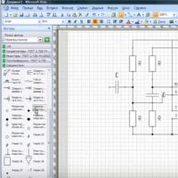 Programs for drawing electrical circuits
 Drawing boards in Sprint-Layout correctly from the first steps
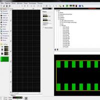 What program can open the file