Excel alternate fixing multiple lines. Loose data fixing method
When working with extensive volumes of tabular data in the Excel program, for reasons, it is necessary to fix a specific section of the table - a header or data that must be constantly located before your eyes, no matter how far the table is scrolling.
Work with Excel 2003
This feature is available in each Excel version, but due to the difference in the interface and location of menu items and individual buttons is not configured equally.
Fastening string
If you secure the header in the file, i.e. The top line, then in the "Window" menu, you should select "Fasten the Area" and select the first column cell of the next line.
To fix multiple lines at the top of the table technology, the extreme on the left of the cell is highlighted in the following fixed lines.
Fastening column
The fixation of the column in Excel 2003 is in the same way, only a cell is highlighted in the top line following the fixed column or several columns.
Fixing the region
The Excel 2003 software package allows you to fix both the columns and lines of the table. To do this, select the cell following the fixed. Those. To fix 5 lines and 2 columns choose the cell in the sixth row and the third column and click "fasten the area".
Work with Excel 2007 and 2010
Late versions of the Excel software package also allow you to lock the file cap on site.
Fastening string
For this:

When it is required to fix not one, but another number of lines, it is necessary to select the first scrolling line, i.e. The one that will be immediately enshrined. After that, everything in the same paragraph is chosen to "fix the area". 
Important! The function of fixing the sections of the table in Excel 2007 and 2010 is significantly finalized. In addition to the fact that it is now not in the "Window" section, and in the section "View", the ability to separately fix the first column or the first line. At the same time it does not matter, in which cell is the cursor, the desired string / column will still be fixed.

Fastening column
To fix the column in the section "Fasten areas" it is necessary to note the option of fixing the first column. 
If you need to save several table columns visible when scrolling, then by analogy with the previous clause, the first scrolled column is distinguished and the "Fasten area" button is pressed. 
Fixing the region
The two options mentioned above can be combined, making it so that when scrolling the table horizontally and verticals will remain on the spot the necessary columns and lines. For this, the first scrolling cell is highlighted by the mouse. 
After, lock the area. 
Those. If, for example, the first line and the first column are fixed - it will be a cell in the second column and the second line, if 3 lines and 4 columns are fixed, then select the cell in the fourth line and the fifth column, etc., the principle of operation should be Cancel.
Important! If there are several sheets in the file, then the part of the table is fixed and the pinch will have to be removed on each separately. When you press the buttons that fix columns, lines and sections of the table, the action is performed only on one sheet, active (ie, open) at the moment.
Cancellation
It happens that fixing a part of the table is required only for the time of filling, and upon subsequent use it is not necessary. It is as easy as a string or column fixed, fixation is canceled.
In Excel 2007 and 2010, this feature is located in the same section "View" and the "Fixing Region" paragraph. If there is some fixed area - a column, a string or a whole area, then a button "Remove the pinning areas" button appears, which removes the entire fixation of the table elements onto the entire sheet. 
Remove the fixation will not partially. For this, you will have to initially cancel fixation everywhere, and then fix on the new required sections of the table.
Output
Fixing elements is a useful feature that greatly facilitates and simplifies work with extensive tables. This function is configured.
Working with multi-page documents in Excel is complicated by the fact that the cells used are often removed from the names of the table blocks for a considerable distance. Constantly scrolling the sheet from the titles to the necessary data is irrational, long and inconvenient. Eliminate this deficiency will help the fixation function. To secure a string in Excel, a minimum of time is required, as a result, the cap in the table will remain in the field of view all the time, regardless of how far cells are lowered with information. Vertical you can make a static column when scrolling.
Loose data fixing method
You can fix you as one and several horizontal blocks at once. To do this, it is necessary:If necessary, fix two or more upper portions horizontally, the following should be done:

Method for fixing vertical blocks when scrolling
To establish immobility of the first vertical band, it is necessary:
Similar to the option with the Horizontal cap, the function of imparting immobiles is implemented by several vertical blocks.

How to make fixed lines and columns together
To fix one or more horizontal bands and vertically at the same time, passing the steps: 
How to remove fixation
Discusing the fixation to be needed to you during the error assumption, or erroneous action in previous lists, in other matters, the procedure is similar:
Now the fixed bands do not remain in any directions. The complexity of the work consists in the order of action and attentiveness.
For convenience of working with large tables, partially leaving the working window, many users will be interested to know how to leave in sight headlines and signatures of individual areas. A number of features should be taken into account:
- Selection of areas is possible in the upper and left part of the sheet. The "Fixing Region" function does not apply to cells placed in the document center.
- When using the cell editing mode (when entering the formula or data into the cells), protection of the document or posting the page, the command for fixing areas is not available. To exit the editing mode of individual items, press the "Enter" or "ESC" button.
- It is allowed to fix the top line of the sheet, left column or several rows and columns simultaneously. For example, when fixing a string 1, and after the column A, the string 1 will remain loose. This operation was required simultaneously.
How to fix the string?
When fixing the formula, timeline, cells and notes, fixed elements are separated using a solid line. This determines the possibility of expanding them separately from each other.

To secure the line there is a number of actions:
- Creating a new program document (or launching an existing one).
- Allocation of the row fixed. To quickly highlight a large string, activate the initial cell, clamp the Shift button and bring to the final item. This ensures the instant allocation of the entire string.

- Then you need to go to the standard tab "View" located in the main window on the toolbar.
- Find the window parameter panel and select the "Secure Area" command. In the proposed list, select the Line fixation function.

This option contributes to the convenience of highlighting the table cap. When viewing the photo it can be seen that the display of fixed rows is made after the tables scrolling until the 200th line.

How to fix columns?
Those who wish to learn how to fix the column in Excel when scrolling the version of the Starter version, should be ready for the lack of this option in the program, users of other Ekel applications (2007 or 2010, 2013), just perform several steps:
Selects the columns of the table.

In the View tab, find the section to secure the areas and fix one or more speakers.

In the future, the table is available to the flushing from right to left. The fixed column will be constantly in the visibility zone.

To cancel previously fixed items, it is necessary to follow a number of instructions:
- Open the View Window on the toolbar.
- Remove the fixation of the areas through the menu in the "Secure Elements" tab.

How to fix the area of \u200b\u200bthe document?
Fastening separately taken groups (from rows and columns) simplifies an overview of complex tables and reports. Simultaneous consolidation of several components of the table is made by highlighting and activating the "Fasten area" button.

The selected areas will remain in a prominent place when scrolling the windows in different directions.
How to divide the window to separate independent areas
To separate the document to separate zones used to work independently of each other, you should activate the "Fixing Region" button, without highlighting the file items. This will ensure the instant separation of the sheet on 4 conventional windows.

Selection of regions
To highlight:
Separate cells - activate them or apply arrows to go to the desired item.
Range of cells - click on the first element of the area of \u200b\u200binterest and drag the mouse pointer to its last element. Or holding the Shift button to use the arrows to increase the selected zone. It is possible to highlight the first cell of the range, followed by pressing the F8 key (instead of holding the SHIFT button) to increase the selected area using the arrows. To prevent increasing the selected area, you should additionally click on the F8 button.
All Document Cells - set the command to "Allocate everything". Press the "Select All" button or use the Ctrl + A buttons. It is important to know that the activation of the Ctrl + A keys on a sheet containing information will be selected the current range. When you restart the Ctrl + A buttons, the entire sheet is allocated.

Unbendable sites - click on the first element or area, holding the Ctrl button and select other cells or ranges. An alternative option will be the selection of the first element, followed by pressing the SHIFT + F8 buttons to add to the designated portion of other non-negative cells or ranges. To prevent the cells and ranges, it is required to start the SHIFT + F8 buttons. It is important to remember the impossibility of canceling individual sections of areas without preventing general selection.
Rows or speakers completely - click on the name of the string (1) or column (2).

Related ranges - carry out the mouse over their names or highlight the first line / column. Then, by holding the Shift button, it remains to activate the last line or column.
Non-dimensional rows or columns - click on the header of the first line or column, then clamping the Ctrl button, click on the names of the speakers or rows provided for the selection.
The cells (at the beginning or end of the lines or column) - click on the cell and clamp Ctrl + arrow.
The site to the last cell of the document where data is contained (on the right in the lower corner) - click on the first cell and hold the Ctrl + Shift + End keys to increase the selected area to the last filled item (right in the corner).
Increasing or decreased cells relative to the existing number in the selected area - by pressing the SHIFT key, activate the last cell provided for adding to the new selected zone.
Reviews
Irina Stolyarchuk, 26 years old, Novosibirsk
For operational calculations of forecasts in Exeme, I often communicate to a link to individual elements or their ranges in the formula. When stretching the formula, the link link remains stationary. So, I need to calculate the cooph. January seasonality, I share the average monthly sale at the average performance for 3 years. When stretching the cell down to count the coefficient. The rest of the months, in February, the average annual sales indicators will be equal to "0".
I highlight the link to the formulas to the formula.


If you click on the "F4" button, the link will appear $ F4:

This makes it possible to learn about the fixation of the column F and its immobility in the process of flushing the formula, and the link to the line 4 will be active.


To secure the range, I highlight it in the Eksel formula and click on the "F4" button.

Olga Trutova, 31 years old, Krasnoyarsk
I like everything in the "smart tables", except for one negative point - they stop being "smart", it is only worth installing a sheet protection, while leaving the table area is not protected. Otherwise, the functions of fixing areas is a convenient tool for filling the forms and summary tables. I work with the Excel 2003 application. To secure tables, you need to open the "Window" tab and select the appropriate command.

Tatyana Sotnikova, 21 years old, Sochi
Zhelel 2013 was downloaded and immediately tested the tool. Allocated fixed cells, then in the "View" tab, click on the "Fasten area" button and the menu that opens selected the consolidation method. At first there were difficulties, since I forgot to exit the edit mode, I had to close the document and return to the previous version. If you again try everything turned out, and when moving a sheet with data up or down, I always see fixed cells.
Video
In this lesson, I will tell you how to fix a string or column in Excel. The fastened areas will always be visible on the screen with a vertical or horizontal scrolling.
Let's start with the easiest one - you will learn to fix one line or one column. It is very easy to do. We go into the tab View -\u003e Fasten the Area. Next, from the drop-down list, choose the necessary action Secure the top row or Secure the first column.
A little more complicated when we need to secure more rows or columns than one. Suppose you need to secure 2 top strings. For this, we highlight 3 string by clicking on its number on the side.


At the border between the second and third line, a special separation will appear.

This means that the strings are fixed and when scrolling the document will stay in place.

Similarly, you can also fix column. To do this, select the column that is next for the fixed, and click on To fix areas. In my example, this is the second column.

Please note that it is impossible to simultaneously fix rows and columns, something one.
In order to remove the fixed areas just go to View -\u003e Fasten the Area and from the drop-down list, select Remove the fixation of the regions.

Congratulations, now you know how to secure the string in Excele.
In this lesson, I will tell you how to set up the date and text in Excel. Suppose you have several cells, one of which is the date. It is necessary to get a cell in which the record "Treaty No. 15 of 28.12.2015" will be stored, provided that the type of document, its number and date will be stored in different cells.
In the past lesson, I already told how to remove duplicates using a special function that appeared from 2007 version. Today we will talk about the possibility that is suitable for earlier versions. We will use an extended filter.
In this lesson, consider the Excel functions that are in the status bar. The status bar in Excel is represented by a strip at the bottom of the program window where additional information can be displayed.
Thanks to the high performance Excel, you can store and work with data in millions of rows and columns. However, strolling all these numerous cells down, to 26935 row it is fairly easy to lose the connection between the values \u200b\u200bin these cells and their meaning. This is one of the reasons why Excel has prepared a special tool for us - FREEZE. (Fasten).
This tool allows you to scroll through cells with information and see the headings of strings and / or columns that are fixed and cannot scroll together with the rest of the cells. So, what button you need to click, and what underwater stones here exist?
How to keep headlines visible
If you have a regular table with one string in the title, then actions are very simple:
- Look at the top line with headers and make sure this line is visible. In this case, the row itself can not be allocated.
The function under consideration has one feature: it fixes the upper apparently string.
Whenever you secure rows or columns, team Freeze Panes. (Fasten the area) turns into a command Unfreeze Panes. (Remove the assignment of areas), which allows you to quickly unlock rows or columns.
How to fix a few rows and / or columns
Increasingly, and more often I meet the tables that have several lines in the title. These are complex structures, but they allow you to place a more detailed text in the headers, thereby clearer to describe the data in the table.
In addition, the need for fixing multiple lines occurs when you need to compare a specific area with data with another area, which is located several thousand rows below.
In such situations, the team Freeze Top Row (Secure the upper line) will not be very useful. But the ability to fix the whole area immediately - this is the most!
This is how it is done:

As always, this is not the end of the story. Many novice users often complain that this technique does not work. This may occur if you have previously fastened some kind of area.
If any of the rows or columns are already fixed, then instead of a team Freeze Panes. (Fasten the area), you will see Unfreeze Panes. (Remove the consolidation of areas). Take a look at the command name before trying to fix the strings, and everything will work as needed.

Use this small, but very convenient tool so that the headers of the areas remained visible. In this case, when scrolling the sheet, you will always know what data before you.
 Magnetometry in the simplest version The ferrozond consists of a ferromagnetic core and two coils on it
 Effective job search course search
 The main characteristics and parameters of the photodiode
 How to edit PDF (five applications to change PDF files) How to delete individual pages from PDF
 Why the fired program window is long unfolded?
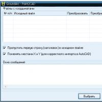 DXF2TXT - export and translation of the text from AutoCAD to display a dwg traffic point in TXT
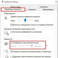 What to do if the mouse cursor disappears