OpenOffice: Calc for beginners. Work with data. Transferring text strings in cell LibreOffice Word Transfer in Cell
Three types of data are introduced into the table cells: text, number, formula. According to the first character, Calc determines that it is introduced: if it is a letter or apostrophe, then this is the text if the number is the number if the equal sign is a formula. To enter data, you need to move to the desired cell, dial data and press ENTER or the cursor move key on the keyboard. Data in cells are edited in several ways:
1) by pressing the left mouse button and fill it, and the previous data will be removed;
2) by pressing the cell with the left mouse button and function key F2 on the keyboard, while the cursor flies in the cell at the end of the word;
3) by pressing twice to the cell with the left mouse button (similar to Pressing F2).
To select the data format, you must use the command Format\u003e Cells\u003e Numbers And then specify the desired format (Fig. 17).
If the text is not included in the cell, then choose one of the ways:
- push the boundaries of the cells horizontally, getting the cursor to the border between the column letters (the arrow of the cursor turns into a bidirectional arrow), and while holding down left key mice shifting the border to the required distance;
- we combine several cells and write text in them. To do this, select several adjacent cells and choose the path through the main menu: Format\u003e Combine Cells (do the same through the toolbar);
- we organize the transfer of text in the cell according to: Format\u003e Cells\u003e Alignment\u003e Transfer according to (Fig. 18).

If the number is not included in the cell, Calc displays it either in exponential form (1230000000 - 1.23E + 09), or instead of the number puts the signs ####. Then push the borders of the cell.
The double click of the left mouse button on the cell entered entered into the data editing mode. In this case, the pointer acquires the view vertical line (cursor).
The transition to the data editing mode will also carry out the click on the input row.
Similarly, we carry out other cell settings. Consider more detail Format\u003e Cells. The first tab of the number (see Fig. 17) allows you to select the data format and setting the selected format, for example, the numeric format allows you to specify number of initial zeros, fractional part , the possibility of separation to discharge, allocation of different color negative numbers. Viewing different formatsWe will see the settings produced for them.
The following tabs are Font and Effects font (Fig. 19 and 20).


Tab Alignmentbriefly described in Fig. eighteen.

To framing the table, perform the following settings:
- Line position: The predetermined style is selected, which will be applied. For this purpose there is also a button Frameon the toolbar Formatting.
- Line: Select the style of the border to be used. This border applies to the borders selected in preview. On the toolbar Formattingyou can also add a button. Line style. Indicate here Color linewhich will be used for selected borders.
- Indentation from content, That is, the size of the interval that will be left between the boundary and the contents of the selection, from the specified side. The use of the same interval to the contents to all four borders when entering a new distance we carry out by installing a tick near Synchronize.
- Shadow style: The shadow effect is applicable to the boundaries. To achieve the best results, we use this effect only when all four borders are visible. Here you choose Position, Widthand Colorshadow
To select the pouring cells, you must specify the color that will be displayed in the sample (field on the right).
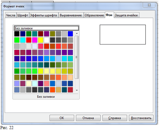
The last tab is Cells (Fig. 23). We specify the following parameters:
Protection:
- Hide everything - We hide the formulas and content of selected cells.
- Protected- Forbid changing the selected cells.
- Hide formulas - We hide the formulas in the selected cells.
Print:
- The sheet print parameters are determined. Hide under seals - Ban the seal of the selected cells.

Leave your comment!
Training course - Basics of work in OpenOffice
Text Editor - OpenOffice Writer
Transportation of gears
For greater readability of the document, you can use the leveling of paragraphs on the left and right edges, but this is not always acceptable - in this case, the distance between the characters in the text increases, which is especially noticeable if there are long words in the text; Of course, it is best to use the transfer.
To OpenOffice.org Writer. had the opportunity to put transfer in the text, you need to install in the properties of the language Russian (menu Service-\u003e Parameters ...-\u003e Setting up language-\u003e Languages, Field "Western").
Transportation of gears can be automatically or manually.
Automatic transfer arrangement is set in the properties of the paragraph - in the installation of the properties of the paragraph style properties on the tab Position on the page In chapter Transportation of gears You need to enable the option Automatically.
For the arrangement of soft (recommended) portes, you need to set the cursor to the place where you can make the transfer and insert the soft transfer symbol by the key combination Control + minus. You can search for all words that can be transferred using the function. Transportation of gears on the menu Service.

Sign "=" means the place of possible transfer; "-" Indicates the place in which it will definitely be produced. To set the transfer, click on the button. Tolerate; To stop the port arrangement, the button is the button Cancel.
Use the button Remove The previously established word transfer is removed.
If you need to never tolerate the word, you need to add it to the dictionary with a sign "=" in the end.
Standard text set rules in Calc cells do not allow you to type text in several lines. And press the ENTER key, habitual for writer programs, only leads to the transition to the next cell. Placing text on strings can be set both after its dial and in the process. In the first case, the cell text will consist of one paragraph, and in the second - from several.
How to set a few lines of text, without creating paragraphs in this case, the text in the cell will consist of one paragraph, and the number of its lines will depend on the width of the cell.
2. Open the Format menu and in the Command list, select Cell.
3. In the Cell format window, on the Alignment tab in the Group on the Activate item to transfer the item according to the words.
In the future, adjusting the width of the column, you can achieve the desired number of text rows in the cell. How to set a few lines of text, creating paragraphs in the second version each line in the cell is a separate paragraph, and the number of strings will remain unchanged with any column width.
1. In the open sheet window, type the first string of the text in the desired cell.
2. At the end of the string to go to the second line of the text, use the CTRL + ENTER key combination.
3. If necessary, apply this shortcut of the keys to create the following rows in the cell.
At the end of the last line Ctrl + Enter should not be used, as it will affect the alignment of the text along the vertical. How to change the color of the font in the cell
2. Open the Font Color button on the Formatting panel.
3. In the open palette, click on the raid the desired color. Conditional format of cells when creating documents and repeated formatting a large number of cells can be used next setting Calc - conditional formatting, that is, by making a certain format to the cell when performing a special specified condition. However, if the style for the cell is installed, it does not change. You can set three conditions for comparing the values \u200b\u200bor formulas in the cells that are checked in order from the first to third conditions. If the first condition coincides, the corresponding style is applied, the second condition is the next designated style. How to configure conventional formatting To use conditional formatting, you must first set up. 1. In the open table window, expand the service menu.
2. In the command list, Mouse over the Cell Content Item.
3. In the Advanced Menu, activate the Calculation item automatically. How to use conditional formatting using this instruction can be defined for each cell to determine up to three conditions for which one or another format is applied to it.
1. In the open sheet window, highlight the desired cells.
2. Open the format menu and select Conditional Formatting.
3. In the Conditional Formatment window, activate the value of Condition 1 and in the first list, select:
Cell value - if conditional formatting depends on the cell value. Select the desired condition in the list on the right: Equally, less, more, etc. And then in the field - link, value or formula;
Formula - If conditional formatting depends on the result of the formula. When you select this value, enter a link to the cell in the field to the right field. If the value of the cell reference is different from zero, the condition is considered to be executed.
4. In the Cell Style list, select Style (Basic, Title, etc.) for use with the specified condition.
5. Close the window with the OK button. How to quickly transfer the conditional formatting to other cells
1. In the open sheet window, highlight the cell with the created conditional formatting.
2. Click the Copy Formatting button on the Standard panel.
3. When the left button is pressed, drag the cursor over the desired cells to which the conditional formatting needs to be applied. Graphic formatting of cells Graphic formatting of cells includes the design of the boundaries of the cells and the fill of their background. How to set the fill of the background the default cell in Calc is used white cell background color. However, if necessary, the color of the fill can be changed.
1. In the open table window, highlight the desired cell or range of cells.
2. Open the Background Color Buttons Menu on the Formatting Panel.
3. In the open palette, click on the desolted color. How to quickly set the boundaries of the cells
1. In the open table window, highlight the desired cell or range of cells.
2. On the Formatting Panel, open the Frame button.
3. In the list, click on the button of the desired frame. How to ask extra options Framing of cells
1. In the open sheet window, highlight the desired range cells.
2. Open the Format menu and in the Command list, select Cell.
3. In the Cell format window on the Frame tab, select the color, frame style, as well as the shadow position.
4. In the content indentation group, set the internal fields with the regulators.
5. Close the window with the OK button.
 Lighting devices based on alternating current LEDs find their niche and may come out beyond its limits.
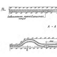 Requirements and rates for cable laying in Earth Scope of application, Definitions
 Automobile stroboscope from laser pointer
 Order 20 UAH to the account. How to Borrow on MTS. Additional information on the service
 How to check the account replenishment
 How to get a loan on tele2?
 Responsiveness SSD on a miniature board What SSD Drive Buy