Reflected transmitter power. On the antennas, coaxial cables and CWS, is simple about complex. What antennas are usually used on the Civil Range
The device for measuring the quality of the feeder coordination with the antenna (CSW-meter) is an indispensable part of the amateur radio station. How reliable information about the state of antenna farm gives such a device? Practice shows that not all the factory manufacturing CSW meters provide high measurement accuracy. To an even greater degree, this is true when it comes to homemade structures. In the readers offered to readers, the article discusses the CSW meter with a current transformer. The devices of this type were widespread from both professionals and radio amateurs. The article presents the theory of its work and analyzed the factors affecting the accuracy of measurements. It completes its description of two simple practical designs of the KSW meters, the characteristics of which will satisfy the most demanding radio amateur.
A bit of theory
If a homogeneous connecting line (feeder) connected to the transmitter with the Zo wave resistance is loaded to the resistance of ZN ≠ Zo, then it occurs both incident and reflected wave. The reflection coefficient g (reflection) is generally determined as the ratio of the amplitude reflected from the wave load to the amplitude of the incident. The reflection coefficients in the current r, and on the voltage RU are equal to the ratio of the corresponding values \u200b\u200bin the reflected and incident waves. The phase of the reflected current (with respect to the falling) depends on the relationship between ZN and Zo. If zn\u003e zo, then the reflected current will be anti-phase incident, and if Zn The value of the reflection coefficient R is determined by the formula where RN and XN - respectively, the active and reactive components of the load resistance at a purely active load of the XN \u003d 0 formula simplified to R \u003d (RN-ZO) / (RN + Zo). For example, if a cable with a wave resistance of 50 ohms is loaded with a resistor resistance of 75 ohms, then the reflection coefficient will be R \u003d (75-50) / (75 + 50) \u003d 0.2. In fig. 1, and the voltage distribution Ul and current Il along the line is for this case (losses in the line are not taken into account). The scale along the ordinate axis for the current is adopted in Zo times more - at the same time, both graphs will be the same vertical size. Dotted line - voltage graphics UH and current IO in the case when Rn \u003d Zo. For example, a portion of a line of λ is taken. At a larger length, the picture will be cyclically repeated every 0.5λ. At those points of the line, where the phases of the falling and reflected coincide, the voltage is maximally and equal to the Max - \u003d Used (1 + R) \u003d Used (1 + 0.2) \u003d 1,2U, and in those where the phases are opposite - the minimum And equal to Ul MIN \u003d Used (1 - 0.2) \u003d \u003d 0.8Ul. By definition of the CWP \u003d UR MAX / / UL MIN \u003d 1L2ULO / 0I8U \u003d 1I5. The formulas for calculating the KSV and R can be written as follows: KSV \u003d (1 + R) / (1-R) \u200b\u200band R \u003d \u003d (KSV-1) / (KSV + 1). We note an important point - the sum of the maximum and minimum stresses Ul Max + Ul MIN \u003d Used (1 + R) + Used (1 - R) \u003d 2UNO, and their difference Ul Max - Ul MIN \u003d 2Ulo. Using the obtained values, it is possible to calculate the power of the incident wave of RPAD \u003d UH2 / ZO and the power of the reflected wave Potr \u003d \u003d (RUO) 2 / ZO. In our case (for KSV \u003d 1.5 and R \u003d 0.2) the power of the reflected wave will be only 4% of the power of the incident. Definition of CWW on the measurement of voltage distribution along the line site in search of values \u200b\u200bUl Max and Ul MIN was widely used in the past not only on open airlines, but also in coaxial feeders (mainly at VHF). To do this, the measuring section of the feeder was used, having a long longitudinal slot, along which a cart was moved to the probe inserted into it - the head of the RF Voltmeter. The CWC can be determined by measuring the current I in one of the wire wires on a portion of less than 0.5λ. Determining the maximum and minimum values, calculate the CWS \u003d IMAX / IMIN. To measure the current, the current-voltage converter is used in the form of a current transformer (TT) with a load resistor, voltage on which is proportional and simulating the current current. We note an interesting fact - with certain parameters TT at its output, it is possible to obtain a voltage equal to the voltage on the line (between the conductors), i.e. UTL \u003d ILZO. In fig. 1, B are shown together a schedule of a change along the line and a graph of the UTL change. Graphs have the same amplitude and shape, but shifted one relative to another by 0.25x. Analysis of these curves shows that it is possible to define M (or CWS) with a simultaneous measurement of the values \u200b\u200bof UR and UTL anywhere. At the places of the maxima and minima of both curves (points 1 and 2), this is obvious: the ratio of these values \u200b\u200bUR / UTL (or UTL / UR) is equal to the CWP, the amount is 2 eo, and the difference is 2RULO. At intermediate points, UR and UTL are shifted in phase, and they need to be added already as vectors, however the above ratios are preserved, since the reflected voltage wave is always inversely in phase the reflected current wave, and RULO \u003d RUTLO. Therefore, a device containing a voltmeter, a calibrated current-voltage converter and a deduction scheme, will determine the parameters of the line as R or CWS, as well as the RPAD and ROTR when it is turned on anywhere. The first information about the devices of this kind refer to 1943 and reproduced in. The first-known author's practical devices were described in. The option of the scheme taken as the basis is shown in Fig. 2. The device contained: The secondary winding of the T1 transformer is included in such a way that when connecting the transmitter to the left according to the connector circuit, and the load is to the right, the total voltage of UC + UT comes to the VD1 diode, and the VD2 diode is different. When connecting to the yield of the KSV meter of the resistive reference load with a resistance equal to the wave resistance of the line, the reflected wave is missing and, therefore, the Voltage on VD2 may be zero. This is achieved in the process of balancing the device by equalizing UT and UC voltages using a C1 trimmed condenser. As was shown above, after such a setting, the value of the difference voltage (with Zn ≠ Zo) will be proportional to the reflection coefficient of the G. Measurement with real load produce so. First, in the SA1 switch position shown on the scheme ("Fading Wave"), the R3 calibration variable resistor is set to the device for the last division of the scale (for example, 100 μA). The SA1 switch is then transferred to the lower position ("reflected wave") and count the value in relation to the case with Rh \u003d 75 Ohm, the device must show 20 μA, which corresponds to R \u003d 0.2. The value of the KSW is determined by the above formula - KSV \u003d (1 +0.2) / / (1-0.2) \u003d 1.5 or KSV \u003d (100 + 20) / / ((100-20) \u003d 1.5. In this example, the detector is assumed to be linear - in reality it is necessary to introduce an amendment that takes into account its nonlinearity. With the appropriate calibration, the device can be used to measure falling and reflected power. The accuracy of the KSV meter as a measuring device depends on a number of factors, primarily on the accuracy of the device balancing in the SA1 position "Reflected Wave" at RN \u003d Zo. The ideal balancing corresponds to the voltages of UC and UT, equal in size and strictly opposite by phase, i.e. their difference (algebraic amount) is zero. In the real design, the unbalanced remnant UOS is always. Consider on the example, as affected by the final result of measurements. Suppose that at balancing it turned out the voltages of Us \u003d 0.5 V and UT \u003d 0.45 V (i.e., the loss of 0.05 B, which is quite real). With a load of RN \u003d 75 Ohm in the 50-ohmic line, we really have a CW \u003d 75/50 \u003d 1.5 and R \u003d 0.2, and the value of the reflected wave, recalculated to the internal abstract levels, will be RUC \u003d 0.2X0.5 \u003d 0, 1 V and RUT \u003d 0.2X0.45 \u003d 0.09 V. Re-turn to Fig. 1, b, the curves on which are given for the CSW \u003d 1.5 (the curves Ul and UTL for the line will in our case, correspond to UC and UT). At point 1 Us Max \u003d 0.5 + 0.1 \u003d 0.6 V, UT min \u003d 0.45 - 0.09 \u003d 0.36 V and KSV \u003d 0.6 / 0.36 \u003d 1.67. At point 2utmax \u003d 0.45 + 0.09 \u003d 0.54 V, Ucmin \u003d 0.5 - 0.1 \u003d 0.4 and KSV \u003d 0.54 / 0.4 \u003d 1.35. From this simple calculation, it can be seen that, depending on the place of inclusion of such a KSV meter in a line with a real KSV \u003d 1.5, or when the line length changes between the instrument and the load, different KSV values \u200b\u200bcan be read - from 1.35 to 1.67! What can lead to inaccurate balancing? 1. The presence of voltage of the cut-off of the gerony diode (in our case, VD2), in which it ceases to be carried out - approximately 0.05 V. So under UOct< 0,05 В
прибор РА1 покажет "ноль" и можно допустить ошибку в балансировке. Относительная
неточность значительно уменьшится, если поднять в несколько раз напряжения Uc и
соответственно UT. Например, при Uc = 2 В и UT = 1,95 В (Uост = 0,05 В) пределы
изменения КСВ для приведенного выше примера будут уже только от 1,46 до 1,54. 2. The presence of frequency dependence of UC or UT voltages. In this case, accurate balancing can be achieved not in the entire range of operating frequencies. We will analyze on the example one of the possible causes. Suppose, a condenser is used in the device C2 Capacity 150 PF with wire outputs with a diameter of 0.5 mm and 10 mm long. The measured inductance of the wire of such a diameter with a length of 20 mM was equal to L \u003d 0.03 μH. On the upper operating frequency f \u003d 30 MHz the resistance of the condenser will be xc \u003d 1 / 2πfs \u003d -j35.4 Ohm, the total reactive resistance of the conclusions XL \u003d 22πFL \u003d J5.7 Ohm. As a result, the resistance of the lower shoulder of the divider will decrease to the value -J35.4 + J5F7 \u003d -J29.7 OH (it corresponds to the condenser with a capacity of 177 PF). At the same time, at frequencies from 7 MHz and below the effect of the conclusions is negligible. Hence the output - in the lower shoulder of the divider, impudent capacitors with minimal conclusions should be used (for example, support or passing) and the inclusion of multiple capacitors is parallel. The conclusions of the "upper" capacitor C1 practically do not affect the situation, since XC has a top condenser a few dozen times more than that of the lower. It is possible to obtain uniform balancing in the entire working band of frequencies using the original solution, which will be discussed when describing practical structures. 3.2. The inductive resistance of the secondary winding T1 at the lower frequencies of the operating range (~ 1.8 MHz) can be significantly shunting R1, which will reduce UT and its phase shift. 3.3. Resistance R2 is part of the detector chain. Since according to the scheme, it shunt C2, in the lower frequencies, the division coefficient can get frequency and phase dependence. 3.4. In the diagram. 2 Detectors on VD1 or VD2 in the open state are shunting with its input resistance RBX bottom shoulder of the capacitive divider on C2, i.e. RBX acts in the same way as R2. The influence of RBX is insignificant with (R3 + R2) more than 40 com, which requires the use of the sensitive indicator of the RA1 with a total deviation current of no more than 100 μA and RF voltage on VD1 at least 4 V. 3.5. The input and output connectors of the KSV meter are usually separated by 30 ... 100 mm. At a frequency of 30 MHz, the difference in the voltage phases on the connectors will be α \u003d [(0.03 ... 0.1) / 10] 360 ° - 1 ... 3.5 °. How it can affect the work, demonstrated in Fig. 3, a and fig. 3, b. The difference in circuits on these figures is that the C1 capacitor is connected to different connectors (T1 in both cases is located on the middle of the conductor between the connectors). In the first case, the noncompensated residue can be reduced if you correct the UOct phase using a small parallel capacitor of the SC, and in the second - on the inclusion of a small inductance of LC in the form of a wire loop. This method is often used both in homemade and "branded" KSV meters, but it should not be done. To make sure that it is enough to rotate the device so that the input connector is output. At the same time, compensation, which helped to turn, will become harmful - uoct will increase significantly. When working on a real line with an inconsistent load, depending on the length of the line, the device can get into such a place on the line, where the introduced correction "will improve" the real KSW or, on the contrary, "worsen" it. In any case, there will be an incorrect count. Recommendation - Place the connectors as close to each other and use the original circuit solution below. To illustrate how much the causes considered above, the reasons for the accuracy of the testimony of the KSV-meter, in Fig. 4 shows the results of checking two factory manufacturers. The verification was that the inconsistent load with the calculated KSV \u003d 2.25 was established at the end of the line consisting of a series of successively connected cable segments with Zo \u003d 50 ohm length each by λ / 8. During the measurement process, the full length line was changed from λ / 8 to 5/8λ. Two instruments were checked: inexpensive Brand X (curve 2) and one of the best models - Bird 43 (curve 3). Curve 1 shows true CWS. As they say, comments are superfluous. In fig. 5 shows a graph of measurement error from the value of the D (Directivity) of the KSV meter. Similar graphs for CBW \u003d 1 / KSV are given in. Applied to the design of Fig. 2 This coefficient is equal to the ratio of voltages of the RF on diodes VD1 and VD2 when connecting to the output of the KSV-meter of the load RN \u003d Zo d \u003d 20lg (2U / UOS). Thus, the better it was possible to balance the scheme (the less Uest), the higher D. You can also use the indicator of the indicator of the RA1 - D \u003d 20 X X LG (IPAD / IOTR). However, this value D will be less accurate due to the nonlinearity of the diodes. The graph of the horizontal axis is postponed by the real QCV values, and on the vertical - measured taking into account the error depending on the value of D of the KSV meter. The dotted line shows an example - a real KSV \u003d 2, the device C d \u003d 20 dB will give an indication 1.5 or 2.5, and with D \u003d 40 dB, respectively, 1.9 or 2.1. As follows from literature data, the CSW-meter according to the scheme Fig. 2 has D - 20 dB. This means that without substantial correction, it cannot be used for accurate measurements. The second most important reason for the incorrect testimony of the KSV meter is associated with the nonlinearity of the volt-amps characteristics of detector diodes. This leads to dependence of the testimony from the level of the power supply, especially in the initial part of the RA1 indicator scale. In branded KSW meters, there are often two scales on the indicator - for small and large power levels. T1 current transformer is an important part of the KSW meter. Its main characteristics are the same as in a more familiar voltage transformer: the number of turns of the primary winding N1 and secondary N2, the transformation coefficient K \u003d N2 / N1, the current of the secondary winding I2 \u003d L1 / K. The difference is that the current through the primary winding is determined by the outer chain (in our case it is a current in the feeder) and does not depend on the load resistance of the secondary winding R1, so the current L2 is also independent of the resistance value of the resistor R1. For example, if the feeder zo \u003d 50 ohms passes the power P \u003d 100 W, the current i1 \u003d √p / zo \u003d 1.41 A and when to K \u003d 20, the secondary winding current will be L2 \u003d I1 / K - 0.07 A. Voltage on The outputs of the secondary winding will be determined by the value R1: 2UT \u003d L2 x R1 and at R1 \u003d 68 ohms will be 2ut \u003d 4.8 V. The power of P \u003d (2ut) 2 / R1 \u003d 0.34 W on the resistor. Pay attention to the peculiarity of the current transformer - the less turns in the secondary winding, the greater the voltage at its outputs (at the same R1). The hardest mode for the current transformer is idling mode (R1 \u003d ∞), while the voltage at its outlet increases sharply, the magnetic cure was saturated and heated so much that it can collapse. In most cases, one turn is used in the primary winding. This round may have different forms, as shown in Fig. 6, a and fig. 6, b (they are equal), but the winding in fig. 6, B is already two turns. A separate question is the use of the screen connected to the screen in the form of a tube between the central wire and the secondary winding. On the one hand, the screen eliminates the capacitive bond between the windings than slightly improves the balance of the difference signal; On the other hand, the screen has vortex currents, also affecting balancing. Practice has shown that with the screen and without it you can get approximately the same results. If the screen is still used, it should be made a minimum, approximately equal to the width of the applied by the magnetic core, and connect with a wide short conductor with a housing. The "ground" screen should be done on the middle line equidistant from both connectors. You can use a brass tube with a diameter of 4 mm from telescopic antennas. For CSW meters, ferrite ring magnetic tubes with sizes K12x6x4 and even K10x6x3 are suitable for passing power up to 1 kW. Practice has shown that the optimal number of turns p2 \u003d 20. In the inductance of the secondary winding 40 ... 60 μH, the greatest frequency uniformity (permissible value is up to 200 μg). It is possible to use magnetic lines with permeability from 200 to 1000, while it is desirable to choose a standard size that will ensure optimal inductance of the winding. You can use magnetic pipers and with less permeability, if you apply large sizes, increase the number of turns and / or reduce the resistance R1. If the permeability of the available magnetic pipelines is unknown, if there is an inductance meter, it can be determined. To do this, it should be coated with ten turns on an unknown magnetic core (the twist is considered to measure the induction of the coil L (μg) and substitute this value in the formula μ \u003d 2.5 LDSR / S, where DSR is the average diameter of the magnetic pipeline in cm ; S - core section in cm 2 (example - K10x6x3 DCP \u003d 0.8 cm and S \u003d 0.2x0.3 \u003d 0.06 cm 2). If μ magnetic pipeline is known, the inductance of the winding from N turns can be calculated: L \u003d μN 2 S / 250DCP. The applicability of magnetic lines to the power level of 1 kW and more can be checked at 100 W in the feeder. To do this, it is necessary to temporarily establish a resistor R1, a value of 4 times greater, respectively, the UT voltage will also increase 4 times, and this is equivalent to increasing the passing power by 16 times. Warming up the magnetic pipeline can be checked the power (power on the time resistor R1 will also increase 4 times). In real conditions, the power on the R1 resistor increases in proportion to the growth of power in the feeder. CWS-meters UT1MA The two constructions of the UT1MA KSV meter, which will be discussed below, have a practically the same scheme, but different execution. In the first version (CMA - 01) high-frequency sensor and indicator part separate. The sensor has input and output coaxial connectors and can be installed anywhere in the feeder path. It is connected to a three-wire cable indicator of any length. In the second embodiment (CMA - 02) both nodes are placed in one case. The KSW - meter scheme is shown in Fig. 7 and it differs from the base diagram. 2 The presence of three correction circuits. Consider these differences. In addition, balancing is carried out by a trimmed capacitor included in the bottom shoulder of the divider. It simplifies installation and allows you to apply a low-power low-sized trimmed condenser. The design provides the ability to measure the power of the incident and reflected waves. To do this, the SA2 switch to the indicator circuit instead of an alternating calibration resistor R4 introduces the R5 stroke resistor to which the desired limit of the measured power is installed. The use of optimal correction and the rational design of the device made it possible to obtain a reference coefficient D within 35 ... 45 dB in the frequency band of 1.8 ... 30 MHz. The following details are applied to KSW meters. The secondary winding of the T1 transformer contains 2 x 10 turns (winding in 2 wires) with a wire of 0.35 PEV placed uniformly on the ferrito-B ring K12 x 6 x 4 permeability of about 400 (measured inductance of ~ 90 μg). Resistor R1 - 68 OM MLT, preferably without screw groove on the body of the resistor. When there is a passing power of less than 250 W, it suffices to establish a resistor with a dispersion capacity of 1 W, with a power of 500 W - 2 W. With a power of 1 kW, the R1 resistor can be made up of two parallel resistors with resistance 130 ohms and a capacity of 2 W each. However, if the COP is a meter is designed for a high level of power, it makes sense to increase twice the number of turns of the secondary winding T1 (up to 2 x 20 turns). This will allow 4 times to reduce the required power dissipation of the resistor R1 (while the C2 capacitor should have twice the large capacity). The capacity of each of the capacitors with G and C1 can be within 2.4 ... 3 PF (CT, CTC, CD to operating voltage 500 V with p ≥ 1 kW and 200 ... 250 V with lower power). Capacitors C2 - on any voltage (KTK or other unhinductive, one or 2 - 3 parallel), Capacitor C3 is a small-sized trimming with limits of a capacity of 3 ... 20 PF (PDA - M, CT - 4). The required capacity C2 capacitor depends on The total magnitude of the tip of the tip of the capacitive divider, into which in addition to the capacitors with "+ C1", also C0 ~ 1 PF capacity between the secondary winding of the T1 transformer and the central conductor. The total tank of the lower shoulder - C2 plus C3 at r1 \u003d 68 ohms should be approximately 30 times more than the tank of the upper. Diodes VD1 and VD2 - D311, C4, C5 and C6 capacitors 0.0033 ... 0.01 μF (km or other high-frequency), indicator RA1 - M2003 with a total deviation current 100 μA, A variable resistor R4 - 150 KV SP - 4 - 2M, R4 - 150 comer resistor. R3 resistor has Resistance 10 com - It protects the indicator from possible overload. The magnitude of the corrective inductance L1 can be determined so. When balancing the device (without L1), it is necessary to note the position of the rotor of the rotor of the C3 condenser at 14 and 29 MHz, then drop it out and measure the container in both marked positions. Suppose, for the upper frequency, the container was less than 5 PF, and the total tank of the lower shoulder of the divider is about 130 PF, that is, the difference is 5/130 or about 4%. Therefore, for frequency alignment, it is necessary at a frequency of 29 MHz to reduce the resistance of the upper shoulder also by ~ 4%. For example, when C1 + C0 \u003d 5 PF capacitance resistance xc \u003d 1 / 2πfs - J1100 Ohm, respectively, Xc - J44 Ohm and L1 \u003d XL1 / 2πF \u003d \u003d 0.24MKHN. In the author's devices, the L1 coil had 8 ... 9 turns with a PELSHO wire 0.29. The inner diameter of the coil is 5 mm, the winding is dense, followed by impregnating glue BF - 2. The final number of turns is specified after its installation in place. Initially, it is balancing at a frequency of 14 MHz, then the frequency is 29 MHz and the number of turns of the coil L1 are selected, in which the diagram is balanced on both frequencies at the same position of the C3 stroke. After achieving good balancing on the middle and upper frequencies, the frequency is 1.8 MHz, the variable resistor resistor 15 ... 20 kΩ is temporarily inserted to the resistor R2 and find a value at which Uoct is minimal. The resistance value of the resistor R2 depends on the inductance of the secondary winding T1 and lies within 5 ... 20 kΩ for its inductance 40 ... 200 μH (large resistance values \u200b\u200bfor greater inductance). In the radio ample conditions, most often in the XV-meter indicator use a microammeter with a linear scale and the countdown is carried out according to the QCV \u003d (IPAD + IOT) / (IPAD -IOTR), where i in microamers - the indicator readings in the "incident" and "reflected" modes respectively. It does not take into account the error due to the nonlinearity of the initial portion of the batteries of diodes. Checking the loads of different values \u200b\u200bat a frequency of 7 MHz showed that at a power of about 100 W indicators of the indicator were on average per division (1 μA) less real values, at 25 W - less than 2.5 ... 3 μA, and at 10 W - on 4 μA. Hence the simple recommendation: For a 100-watt variant - to move the initial (zero) arrow position in advance to one division upward, and when using 10 W (for example, when setting up an antenna), add the "reflected" 4 μA to sample. Example - Countdown "Falling / reflected" 100/16 MCA, and the correct KSV will (100 + 20) / (100 - 20) \u003d 1.5. With a significant power - 500 W and more - in the specified correction there is no need. It should be noted that all types of amateur KSW meters (on a current transformer, bridge, on directional axes) give the reflection coefficient R, and the KCV value is then calculated. Meanwhile, it is R is the main indicator of the degree of coordination, and the KSV is an indicator of the derivative. Confirmation of the said may be the fact that in telecommunication the degree of harmonization is characterized by the attenuation of inconsistencies (the same R, only in decibels). In expensive corporate devices, the R called Return Loss is also provided. What will happen if the detectors apply silicon diodes? If a geron diode has a cut-off voltage at room temperature, in which the current through a diode is only 0.2 ... 0.3 μA, it is about 0.045 V, then the silicon already 0.3 V. is therefore to maintain the counting accuracy during the transition to Silicon diodes, it is necessary to raise UC and UT voltages to more than 6 times (!). In the experiment, when replacing D311 diodes on KD522, at p \u003d 100 W, the load Zn \u003d 75 Ohm and the same UC and UT, the numbers turned out: until replaced - 100/19 and CWS \u003d 1.48, after replacement - 100/12 and Calculated KSV \u003d 1.27. The application of the doubling scheme on diodes KD522 gave an even worst result - 100/11 and the calculated CWS \u003d 1.25. The sensor housing in a separate embodiment can be made of copper, aluminum or paved from the plates of the double-sided foil fiberglass with a thickness of 1.5 ... 2 mm. A sketch of such a design is shown in Fig. 8, a. The housing consists of two compartments, in one opposite friend, the RF connectors are located (CP - 50 or SO - 239 with flanges with dimensions 25x25 mm), jumper from the wire with a diameter of 1.4 mm in polyethylene insulation with a diameter of 4.8 mm (from the RK50 cable - 4), current transformer T1, capacitors of the capacitive divider and the compensation coil L1, in the other - resistors R1, R2, diodes, trim and blocking capacitors and a small-sized LC connector. Conclusions T1 minimum length. The connection point C1 "and C1" with the coil L1 "hangs in the air", and the connection point C4 and C5 of the middle output of the XZ connector is connected to the instrument housing. Partitions 2, 3 and 5 have the same dimensions. There are no holes in the partition 2, and in the partition 5, the hole is made under a specific LC connector through which the indicator unit will be connected. In the middle jumper 3 (Fig. 8, b) around the three holes on both sides, the foil is selected, and three passage conductor are installed in the holes (for example, M2 and MZ brass screws). Sketches of sidewalls 1 and 4 are shown in Fig. 8, c. The dotted lines show the location of the connection before soldering, which is for greater strength and ensure electrical contact is made on both sides. To configure and check the KSV - meter, an exemplary load resistor 50 ohms (antenna equivalent) is required with a capacity of 50 ... 100 W. One of the possible ammunition structures is shown in Fig. 11. It uses the common resistor of your resistance 51 Ohm and the dispersion capacity of 60 W (rectangle with dimensions of 45 x 25 x 180 mm). Inside the ceramic housing of the resistor is a long cylindrical channel filled with a resistive substance. The resistor should be tightly pressed to the bottom of aluminum casing. This improves heat removal and creates a distributed capacity that improves extension. Using additional resistors with a dispersion capacity of 2 W, the input load resistance is set in the range of 49.9 ... 50.1 Ohm. With a small correction capacitor at the entrance (~ 10 PF), it is possible on the basis of this resistor to obtain a load with the CWS no worse than 1.05 in the frequency band up to 30 MHz. Excellent loads are obtained from special small-sized resistors of type P1 - 3 with a rating of 49.9 Ohm, withstanding significant power when using an external radiator. Comparative tests of the KSW meters of different firms and devices described in this article were carried out. The check was that the transmitter with an output power of about 100 W through the test 50-ohm xv - the meter was connected to the inconsistent load of 75 ohms (an antenna equivalent to the power of 100 W factory manufacture) and two dimensions were performed. One - when connecting a short cable of RK50, a length of 10 cm, the other - through the RK50 cable with a length of ~ 0.25λ. The smaller the scatter of the readings, the more expensive the device. At a frequency of 29 MHz, the following KSV values \u200b\u200bwere obtained: With a load of 50 ohm at any length of cables, all devices are "friendly" showed KSV<
1,1. The reason for the larger scatter of the RSM - 600 testimony was found to find out when it was studied. In this device, a non-capacitive divider is used as a voltage sensor, but a stress transformer with a fixed transformation coefficient. This removes the "problems" of the capacitive divider, but reduces the reliability of the device when measuring high capacity (the limit power of the RSM - 600 is only 200/400 W). There is no random element in its scheme, therefore the load resistor of the current transformer must be high accuracy (at least 50 ± 0.5 ohms), and the resistor resistor 47.4 ohms was actually used. After it is replaced with a resistor of 49.9 Ohms, the measurement results were significantly better - 1.48 / 1.58. It is possible, with the same reason, a large variation of the testimony of the devices SX - 100 and KW - 220 is associated. Measurement with inconsistent load using an additional quarter-wave 50 - ohm cable - a reliable way to check the quality of the KSW - meter. Note three points: Literature
Standing wave coefficient (KSWN, VSWR) In the modern world, electronic equipment develops with seven-mile steps. Every day something new appears, and these are not only small improvements in existing models, but also the results of the use of innovative technologies that allow you to improve the characteristics. It does not lag behind electronic technology and the instrument-making industry - after all, to develop and release new devices to the market, they must be carefully tested, both at the design and development phase and at the production stage. A new measuring equipment and new measurement methods appear, and, therefore, new terms and concepts. For those who are often faced with incomprehensible abbreviations, abbreviations and terms and would like to understand their meanings deeper, and this rubric is intended. The coefficient of standing wave voltage is the ratio of the largest voltage amplitude line to the smallest. The coefficient of standing wave for voltage is calculated by the formula: , In the ideal case, KSVN \u003d 1, this means that the reflected wave is absent. When the reflected wave appears in direct dependence on the degree of mismatch of the path and the load. The permissible values \u200b\u200bof the KSWN at the operating frequency or in the frequency band for different devices are regulated in technical specifications and GOST. Typically, the acceptable values \u200b\u200bof the coefficient are in the range from 1.1 to 2.0. Measure the KSWN, for example, using the two directional couplers included in the path in the opposite direction. In Space Technology, the KSWN is measured by the CWS sensors built into the waveguide paths. Modern chain analyzers also have built-in KSVN sensors. When performing measurements of the KSWN, it is necessary to take into account that the attenuation of the signal in the cable leads to measurement errors. This is explained by the fact that both falling and reflected waves feel attenuation. In such cases, KSVH is calculated as follows: where k is the attenuation coefficient of the reflected wave, which is calculated as follows: k \u003d 2bl,
After the antenna is installed, it must be configured at a minimum of the KSV value in the middle of the operating frequency portion or if it is assumed to work only at one frequency, according to the minimum value of the KSV at this frequency. Table 1. Power loss with different QCV values Figure 1. Connection diagram of the KSV meter Consider an example of an antenna setting on the average mesh frequency C (frequency 27,205 MHz) by changing the length of the pin. First, you need to measure the KSV value on 1 channel of the S. Mesh. Then on the last (40) Channel C. S. If the KSV value is greater than 3 in both cases, it means an antenna is incorrect, not designed to work in this range or has faults. If the KSV, measured on 1 channel, is greater than the CWV value on 40 channel, then the pin length should be shortened, if on the contrary, the pin must be lengthened (extend from the holder). We get up for 20 channels of the grid C, measure the CWS, remember its value. We unscrew the screws that lock the pin, move it by 7-10 mm in the desired side, tighten the screws that check the CWW again. If the pin is inserted to the limit, and the KSW is still high, it will have to shorten the pin physically. If the pin is put forward to the maximum, then you will have to increase the length of matching the coil. Install the pin in the middle of the mount. We bite 5-7 mm, measuring the CWS, we bite again. At the same time, you follow the value of the CWS decreased. As soon as it reaches a minimum and starts to increase, stop mocking over the pin and then adjust its length by changing the position in the antenna thus we find the minimum of the CWS. Please note that the antenna needs to be configured only at the place of its final installation. This means that, transferred to the antenna to another place, it will need to be configured again. If you received the CWS of about 1.1-1.3, this is an excellent result. If you got the order of about 1,3-1.7, it is also good and nothing to worry about. If KSV is 1.8 - 2, you should pay attention to the losses in the RF connectors (incorrect cutting of the cable, poor conversion of the central cable vein, etc.) for antenna such a level of matching will mean that it has problems with coordination, and She needs customization. KSV 2,1 - 5 means a clear malfunction in an antenna or its incorrect installation. KSV more than 5 means breaking the central cable or in the antenna. From another source The length of the 50-ohm cable in the half-wave, the "half-wave repeater" mode (is true for cables with solid polyethylene insulation of the central core) Number of half feet The average frequency MHz Cable cut length 


Standing wave coefficient (KSWN, VSWR)
where U 1 and U 2 is the amplitudes of the incident and reflected waves, respectively.![]() ,
,
Here in - specific attenuation, dB / m;
L - cable length, m;
And multiplier 2 takes into account the fact that the signal is attenuating when transmitting from the source of the microwave signal to the antenna and on the way back.
What is KSV? KSV - the coefficient of standing wave is a measure of coordination of the antenna-feeder path. It shows the percentage of power loss in the antenna. Power loss with different CWV values \u200b\u200bare shown in Table 1. ATTENTION!!! PRAOP should allow your output power! That is, if the device is designed for the maximum power of 10W, and to supply 100W to the input, the result will be quite obvious in the form of smoke and quite touch the sense of smell. The switch must be put in the FWD position (direct inclusion). Turning on the transmission, you need to set the handle the pointer to the end of the scale. This makes calibration of the instrument readings. Calibrate the device is needed every time when the operating frequency changes. Next, when switching (when transmitted), the device is in the REF position, turn on the transmission and read the value of the KSV on the instrument scale.
Grid "C" Catch "D" Grid "C" & "D"
27.5
1 3.639m 3.580m 3.611m
2 7.278m 7.160m 7.222m
3 10.917m 10.739m 10.833m
4 14.560m 14.319m 14.444m
5 18.195m 17.899m 18.055m
Coefficient of standing wave
Coefficient of standing wave - The ratio of the greatest value of the amplitude of the electric or magnetic field of the standing wave in the transmission line to the smallest.
It characterizes the degree of coordination of the antenna and the feeder (also talk about coordination of the output of the transmitter and the feeder) and is a frequency-dependent value. The reverse value of the KSW is called the CBW - the coefficient of the running wave. The values \u200b\u200bof the KSV and the KSVN should be distinguished (coefficient of standing wave voltage): the first is calculated by power, the second - voltage amplitude and in practice it is used more often; In general, these concepts are equivalent.
The coefficient of standing wave for voltage is calculated by the formula:
Where U 1. and U 2. - amplitudes of falling and reflected waves, respectively.
You can establish a connection between KCBH and the reflection coefficient G:
Also, the value of the coefficient of the standing wave can be obtained from expressions for S-parameters (see below).
In the ideal case, KSVN \u003d 1, this means that the reflected wave is absent. When the reflected wave, the KSW increases in direct regulation on the degree of disagreement of the path and load. The permissible values \u200b\u200bof the KSWN at the operating frequency or in the frequency band for different devices are regulated in technical specifications and GOST. Typically, the acceptable values \u200b\u200bof the coefficient are in the range from 1.1 to 2.0.
The CWV value depends on many factors, for example:
- Wave resistance of microwave cable and microwave source
- Heterogeneity, spikes in cables or waveguides
- Quality of cable cutting in microwave connectors (connectors)
- The presence of transition connectors
- Antenna Resistance at Cable Connection Point
- The quality of manufacturing and setting the source of the signal and the consumer (antenna, etc.)
Measure the KSWN, for example, using the two directional couplers included in the path in the opposite direction. In Space Technology, the KSWN is measured by the CWS sensors built into the waveguide paths. Modern chain analyzers also have built-in KSVN sensors.
When performing measurements of the KSWN, it is necessary to take into account that the attenuation of the signal in the cable leads to measurement errors. This is explained by the fact that both falling and reflected waves feel attenuation. In such cases, KSWN is calculated as follows:
Where TO - The attenuation coefficient of the reflected wave, which is calculated as follows:,
here IN - specific attenuation, dB / m;
L. - Cable length, m;
And multiplier 2 takes into account the fact that the signal is attenuating when transmitting from the source of the microwave signal to the antenna and on the way back. So, when using the cable PK50-7-15, the specific attenuation at the SI-bi frequencies (about 27 MHz) is 0.04 dB / m, then at a cable length of 40 m, the reflected signal will be tightened 0.04 2 40 \u003d 3.2 dB. This will lead to the fact that with the real value of KSVN, equal to 2.00, the device will show only 1.38; With a real value of the 3.00 device will show about 2.08.
The bad (high) value of the load (H) of the load leads not only to the deterioration of the efficiency due to the reduction of the useful power received in the load. Other consequences are possible:
- The failure of a powerful amplifier or transistor, since at its output (collector) are summed up (at worst) the output voltage and the reflected wave, which may exceed the maximum allowable semiconductor transition voltage.
- The deterioration of the unevenness of the frequency response.
- The excitation of the mating cascades.
Protective valves or circulators can be used to eliminate this. But with continuous work on a bad load, they may fail. Matching attenuators can be used for low-power transmission lines.
Communication of KSVN with S-Parameters of the Quadruple
The coefficient of the standing wave can be unambiguously associated with the parameters of the transfer of a four-solubular (S-parameters):
where is the complex reflection coefficient of the signal from the input of the measured path;
KSV analogues in foreign publications
- VSWR - full analog of KSVN
- SWR - full analog of KSV
Notes
Wikimedia Foundation. 2010.
In the line with the CWS\u003e 1, the presence of reflected power does not lead to the loss of transmitted power, although some losses are observed due to the final attenuation in the line in the feeder line without loss no power loss due to reflection regardless of the QCV value. On all Kb bands with a cable having low losses, losses in the incidental line are usually insignificant, but it can be essential to the VHF, and the microwave even extremely large. The attenuation in the cable depends primarily on the characteristics of the cable itself and its length. When working on the KB, the cable must be very long or very bad so that the losses in the cable have become very significant.
Reflected power does not flow back to the transmitter and does not damage it. Damage, sometimes attributed to high CWS, usually causes the output cascade of the transmitter to the incidental load. The transmitter does not "see" the KSW, he "sees" only the impedance of the load, which depends on the CWC. This means that the load impedance can be made precisely corresponding to the desired (for example, using an antenna tuner), without worrying about the CWW in the feeder.
The efforts spent on the reduction of KSV below 2: 1 in any coaxial line are generally presented in the point of view of an increase in the efficiency of the antenna radiation, but are suitable if the transmitter protection circuit is triggered, for example, at CWS\u003e 1.5.
High CWW does not necessarily indicate that the antenna works badly - The effectiveness of the antenna radiation is determined by the ratio of its radiation resistance to the overall input resistance.
Low CWS is not necessarily evidence that the antenna system is good. On the contrary, the low CWW in a wide frequency band is a reason for suspicion that, for example, in the dipole or vertical antenna, the loss resistance due to poor connections and contacts, an inefficient grounding system, loss of cable, moisture in line, etc. Thus, the load equivalent provides in the KSV line \u003d 1.0, but it does not radiate at all, and the short vertical antenna with a radiation resistance of 0.1 Ohms and the resistance loss of 49.9 ohms radiates only 0.2% of the incoming power, while ensuring KSV 1.0 in the feeder.
To achieve maximum RF current and the antenna system does not necessarily have a resonant length And does not require a feeder of a certain length. The essential mismatch between the power line and the emitter does not prevent the absorption of all actually incoming power by the emitter. When using the appropriate matching (for example, an antenna tuner) to compensate for the reactivity of the non-resonant emitter at the site of connecting the feeder line of random length antenna system is consistent, and in fact all the output power can effectively be effectively emissions.
The CWS in the feeder line does not affect the configuration of the antenna tuner installed near the transmitter. The low CWW in the line achieved with the help of the tuner is usually evidence that during the tuner configuration process there was a mismatch between the transmitter and the inlet of the antenna tuner, and the transmitter works on the inconsistent load.
Contrary to mutual ideas, with a good symmetric (balanced) antenna tuner and an open two-wire feeder line, the radiation fed in the center of the dipole with a length of 80 m, operating in the range of 3.5 MHz, not much more efficiently radiation of the same antenna with a length of 48 m, operating in the same range And with the same transmitter power. The efficiency of the radiation of a dipole configured to the resonance at a frequency, for example, 3750 kHz, almost the same as at a frequency of 3500 or 4000 kHz when using any feeder of reasonable length; Although it can be expected that the CWW on the edges of the range can reach 5 and that the coaxial cable will actually work as a customized line. In this case, of course, it will be necessary to use the appropriate coordination device (for example, an antenna tuner) between the transmitter and the feeder. If the coaxial feeder of any antenna system requires a certain length, the same input impedance can be obtained with a cable of any length using an appropriate simple coordination chain from inductors and containers.
High CWW in a coaxial feeder caused by significant mismatch of the characteristic resistance of the line and the input resistance of the antenna, by itself, it does not cause the occurrence of HF current on the outer surface of the cable braid and the emission of the feeder line. In the ranges of short waves, the high KSV in any open line operating with a high QCV will neither cause an antenna current over the line, nor lead to the radiation of the line provided that currents in the line are balanced, and the distance between the conductors of the line is not enough compared to the working The wavelength (this is true and to the VHF, subject to the absence of sharp bends of the line). The current on the outer surface of the feeder braid and the feeder radiation is practically absent if the antenna is balanced relative to the Earth and the feeder (for example, when using a horizontal antenna, the feeder should be located vertically); In such cases, you do not need to use symmetrical devices (balusters) between the antenna and feeder.
KSV-meters installed on the site between the antenna and feeder do not provide more accurate measurement of the CWS. The CWW in the feeder cannot be adjusted by changing the length of the line. If the testimony of the KSV meter is distinguished significantly when moving along the line, this may indicate the antenna feeder effect caused by a current current on the outer side of the coaxial cable braid, and / or on the poor design of the KSW meter, but not that the CWW changes along lines.
Any reactivity added to the existing resonant load (having only active resistance) in order to reduce the CWS in the line, will only cause an increase in reflection. The lowest CWW in the feeder is observed on the resonant frequency of the radiating element and does not completely depend on the feeder length.
The efficiency of radiation of dipoles of various types (from a thin wire, a loop dipole, a "thick" dipole, a trap or coaxial dipole) is almost the same, provided that each of them has minor ohmic losses and is powered by the same power. However, "thick" and looped dipoles have a wider frequency lane compared to an antenna from a thin wire.
If the antenna's input impedance differs from the characteristic resistance of the feeder line, the transmitter load resistance can be very significantly different from the characteristic line resistance (if the electrical length of the line is not multiple L / 2), and from resistance at the connection site to the antenna. In this case, the impedance of the transmitter load depends on the feeder length, which acts as a resistance transformer. In such cases, if a suitable chain of matching between the transmitter and the transfer line is not established, the load impedance can be complex (i.e. have active and reactive components), and with it the output transmitter can not cope with it. In this case, the change in the length of the transmission line is sometimes possible to ensure the negotiation of the load with the transmitter - this is exactly this circumstance, rather than any losses associated with the CWW led to many incorrect ideas about the work of feeder lines.
Any disassembled-length feed in the center of antenna with any type of low loss feeder will provide a fairly effective radiation of electromagnetic energy. At the same time, as a rule, a good antenna tuner is required if the transmitter is designed to work with low-voltage load (for example, 50 ohms). This explains the fact that many years feeding in the center of the dipole remains a popular multi-band antenna.
 Causes of why Flash Player does not work, and troubleshooting
 The laptop itself turns off, what to do?
 HP Pavilion DV6: Characteristics and Reviews
 Format representation of a floating point numbers How negative numbers are stored in the computer's memory
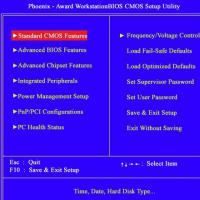 Computer fries and does not turn on what to do?
 Why does not work mouse on a laptop or mouse?
 How to increase or decrease the scale of the page (font) in classmates?