We are using parameters. Using parameters to find the optimal f. Functions with parameters
>> Informatics 7th grade >> Informatics: Eight and command to cycle Repeat N times
Practical robot to subject Informatics class 7.
Look at those: Eight and command cycle Repeat N times
Test: Test Word
Question number 1: What do we use document page settings for?
To insert pagination
To put hyphenations
To set indents from page borders to text borders
To align text
Answer: 3;
Question number 2: Can we draw a frame around part of the text to make it stand out?
Choose one of the answer options:
Yes, you need to use borders and fill for that.
And for this you need to use the page parameters
This can be done using the Fields item in the Page Settings.
No, you can only frame the whole page
Answer: 1;
Question number 3: Attention, there are several possible answers to this question!
What points can we carry out when printing a document?
Specify the number of pages
Specify printing multiple pages on one
Specify to print 5 pages on one
print only individual pages
Select to print multiple copies
Answer: 1,2,4,5;
Question number 4: A text editor is a program for ...
Choose one of the answer options:
Processing graphic information
video processing
processing text information
work with music recordings
Answer: 3;
Question number 5: How to delete a character to the left of the cursor ...
Choose one of the answer options:
Click Delete
Press BS
Press Alt
Press Ctrl + Shift
Answer: 2;
Question number 6: Specify how to save the edited document under a different name.
Question number 7: What action can we perform with the table?
Please select several answer options:
Merging cells
Change the number of rows and columns
Fill one cell
Insert picture instead of border
change the appearance of table borders
Answer: 1,2,3,5;
Question number 8: The cursor is
Choose one of the answer options:
Text input device
keyboard key
smallest display item on the screen
a mark on the monitor screen indicating the position at which keyboard input will be displayed
Answer: 4;
Question number 9: How to enable the Drawing toolbar?
Choose one of the answer options:
View - Toolbars - Drawing
Edit - Paste - Toolbars - Draw
File - Open - Draw
Answer: 1;
Question number 10: How can you insert a picture into a TP MS Word text document?
(Attention to this question, there are several possible answers.)
Please select several answer options:
From graphic editor
from file
from the collection of ready-made pictures
from the File menu
from printer
Answer: 1,2,3;
Question number 11: How in text editor to print a character that is not on the keyboard?
Choose one of the answer options:
Use symbol insertion
Use drawing for this
Paste from special file
Answer: 1;
Question number 12: Specify the sequence of actions to be performed when you insert a formula.
Indicate the order of the answer options:
Select the menu item Insert
Click Object
Select Microsoft Equation
Write a formula
Left-click in a free area of the screen
Answer: 1-2-3-4-5;
Nominated by the teacher of informatics of the International Lyceum "Grand" Cheban L.I.
Calendar-thematic planning in informatics, video in informatics online, informatics in schools
Now that the most suitable values of the distribution parameters have been found, we calculate the optimal f for this distribution. We can apply the procedure that was used in the previous chapter to find the optimal f under normal distribution. The only difference is that the probabilities for each standard value (X value) are calculated using equations (4.06) and (4.12). In a normal distribution, we find the column of associated probabilities (probabilities corresponding to a certain standard value) using equation (3.21). In our case, in order to find the associated probabilities, one should follow the procedure described in detail earlier:
For a given standard X value, calculate its corresponding N \ "(X) using equation (4.06).
For each standard X value, calculate the accumulated sum of the N \ "(X) values corresponding to all previous X.
Now to find N (X) i.e. total probability for a given X, add the current sum corresponding to the value of X to the current sum corresponding to the previous value of X. Divide the resulting value by 2. Then divide the resulting quotient by total amount of all N \ "(X), ie the last number in the column of running sums. This new quotient is the associated 1-tailed probability for a given X.
Since now we have a method for finding associated probabilities for standard values of X at this set parameter values, we can find the optimal f. The procedure is exactly the same as that used to find the optimal f under a normal distribution. The only difference is that we calculate the column of associated probabilities in a different way. In our example with 232 trades, the values of the parameters that are obtained with the lowest value of the K-S statistic are 0.02, 2.76, O and 1.78 for LOC, SCALE, SKEW and KURT, respectively. We obtained these parameter values using the optimization procedure described in this chapter. K-S statistics== 0.0835529 (meaning that at its worst point, the two distributions are 8.35529% removed) at a significance level of 7.8384%. Figure 4-10 shows the distribution function for those parameter values that best fit our 232 trades. If we take these parameters and find the optimal f for this distribution, limiting the distribution to +3 and -3 sigma using 100 equally spaced data points, we get f = 0.206, or 1 contract for every $ 23,783.17. Compare this with the rule of thumb, which will show that optimal growth is achieved with 1 contract for every $ 7,918.04 in the account balance. We get this result if we constrain the distribution to 3 sigma on each side of the mean. In fact, in our empirical trade flow, we had a worst-case loss of 2.96 sigma and a best-case win of 6.94 sigma. Now if we go back and restrict the distribution to 2.96 sigma to the left of the mean and 6.94 sigma to the right (and this time using 300 equally spaced data points), we get the optimal f = 0.954, or 1 contract for every $ 5062.71 on the account balance. Why does it differ from the empirical optimal G = 7918.04?
The problem is the "roughness" of the actual allocation.
Recall that the significance level of our best fit parameters was only 7.8384%. Let's take a distribution of 232 trades and place it in 12 cells from -3 to +3 sigma.
Cells Number of trades
Bg „. -0.5 0.0 43
b - \ "0.0 0.5 69
Note that there are gaps on the tails of the distribution, i.e. areas, or cells, where there is no empirical data. These areas are smoothed out when we fit our regulated distribution to the data, and it is these smoothed areas that cause the difference between the parametric and empirical optimal G. Why is our characteristic distribution, with all the possibilities of adjusting its shape, not very close to the actual distribution? The reason is that the observed distribution has too many inflection points. The parabola can be directed with branches up or down. However, along the entire parabola, the direction of the concavity or convexity does not change. At the point of inflection, the direction of the concavity changes. The parabola has 0 inflection points,
4899,56 -3156,33 -1413,1 330,13 2073,36 3816,59

Figure 4-11 Inflection points of the bell-shaped distribution
Figure 4-10 Adjustable allocation for 232 trades
since the direction of the concavity never changes. An S-shaped object lying on its side has one inflection point, i.e. the point where the concavity changes. Figure 4-11 shows normal distribution... Note that there are two inflection points in a bell-shaped curve such as a normal distribution. Depending on the SCALE value, our adjustable distribution can have zero inflection points (if the SCALE is very low) or two inflection points. The reason our regulated distribution does not describe the actual distribution of trades very well is because the actual distribution has too many inflection points. Does this mean that the resulting characteristic distribution is incorrect? Most likely no. If we wanted to, we could create a distribution function that had more than two inflection points. Such a function could be better fitted to the real distribution. If we were to create a distribution function that allows an unlimited number of inflection points, then we would fit it exactly to the observed distribution. The optimal f obtained from such a curve would practically coincide with the empirical one. However, the more inflection points we would have to add to the distribution function, the less reliable it would be (i.e., it would less represent future trades). We are not trying to exactly fit the parametric IK to the observable, but we are only trying to determine how the observed data is distributed so that we can predict with great certainty the future optimal 1 (if the data is distributed in the same way as in the past). False inflection points have been removed in the regulated distribution, tailored to real trades. Let us explain the above with an example. Let's say we are using a Galton board. We know that the asymptotic distribution of balls falling through the board will be normal. However, we are only going to throw 4 balls. Can we expect that the results of throwing 4 balls will be distributed normally? How about 5 balls? 50 balls? In an asymptotic sense, we expect the observed distribution to be closer to normal as the number of trades increases. Fitting the theoretical distribution to every inflection point in the observed distribution will not give us a greater degree of accuracy in the future. At a large number of trades we can expect that the observed distribution will converge with the expected one and many inflection points will be filled with trades when their number goes to infinity. If our theoretical parameters accurately reflect the distribution of real trades, then the optimal G derived from the theoretical distribution will be more accurate for the future sequence of trades than the optimal G calculated empirically from past trades. In other words, if our 232 trades represent the distribution of future trades, then we can expect that the distribution of future trades will be closer to our "tuned" theoretical distribution than the observed one, with its many inflection points and "noise" due to finite the number of transactions. Thus, we can expect that the future is optimal (it will look more like the optimal G obtained from the theoretical distribution than the optimal G obtained empirically from the observed distribution.
So, it is best in this case to use not the empirical, but the parametric optimal G. The situation is similar to the considered case with 20 coin tosses in the previous chapter. If we expect 60% of winnings in a 1: 1 game, then the optimal G = 0.2. However, if we had only empirical data about the last 20 throws, 11 of which were winning, our optimal (would be 0.1. We assume that the parametric optimal (($ 5062.71 in this case) is correct, since it is optimal for the function that "generates" trades.As in the case of the just mentioned game with a coin toss, we assume that the optimal (for the next trade is determined by the parametric generating function, even if the parametric (differs from the empirical optimal)
Obviously, the limiting parameters have big influence to the optimal Г How to choose these limiting parameters? Let's see what happens when we move the upper border. The following table is compiled for a 3 sigma lower limit using 100 equidistant data points and optimal parameters for 232 trades: \ r \ nUpper limit G \ r \ n3 Sigmas 0.206 $ 23783.17 \ r \ n4 Sigmas 0.588 $ 8332.51 \ r \ n5 Sigmas 0.784 $ 6249.42 \ r \ n6 Sigmas 0.887 $ 5523.73 \ r \ n7 Sigmas 0.938 $ 5223.41 \ r \ n8 Sigmas 0.963 $ 5087.81 \ r \ n * * * \ r \ n * * * \ r \ n100 Sigmas $ 0.999 4904.46 \ r \ n
Note that with a constant lower bound, the higher we move the upper bound, the closer the optimal (to 1. Thus, the more we push the upper bound, the closer the optimal (in dollars it will be to the lower bound (expected worst-case loss)). in the case when our lower border is at -3 sigma, the more we move the upper border, the closer to the optimal limit (in dollars it will be to the lower border, i.e. to $ 330.13 - (1743.23 * 3) = = - $ 4899.56 Look what happens when the upper bound does not change (3 sigma) and we move the lower bound Quite quickly the arithmetic mathematical expectation of such a process turns out to be negative because more than 50% of the area under the characteristic function is on the left from the vertical axis.Therefore, when we move the lower bounding parameter, the optimal (tends to zero. Now let's see what happens if we simultaneously start to move both bounding pairs meters. Here we use a set of optimal parameters 0.02, 2.76, 0, and 1.78 to distribute 232 trades and 100 equidistant data points:
Upper and lower bounds B \ r \ n3 Sigmas 0.206 $ 23783.17 \ r \ n4 Sigmas 0.158 $ 42 040.42 \ r \ n5 Sigmas 0.126 $ 66 550.75 \ r \ n6 Sigmas 0.104 $ 97 387.87 \ r \ n * * * \ r \ n * * * \ r \ n100 Sigmas 0,053 $ 322625,17 \ r \ n
Note that the optimal (approaches 0 when we push back both limiting parameters. Moreover, since the worst-case loss increases and is divided by the smaller optimal G, our $ 1, i.e. the amount of funding of 1 unit, is also approaching infinity.
Problem the best choice restrictive parameters can be formulated as a question: where can the best and worst trades happen in the future (when will we trade in this market system)? The distribution tails actually tend to plus and minus infinity, and we should fund each contract with an infinite amount (as in the last example, where we pushed both boundaries). Of course, if we're going to trade endlessly long time , our optimal (in dollars it will be infinitely large. But we are not going to trade in this market system forever. The optimal G at which we are going to trade in this market system is a function of the best and worst trades assumed. Remember if we flip a coin 100 times and write down the longest bar of tails in a row, and then flip the coin 100 more times, then the bar of tails after 200 tosses is likely to be greater than after 100 tosses. In the same way, if the worst case loss in our history of 232 trades was 2 , 96 sigma (let's take 3 sigma for convenience), then in the future we should expect a loss of more than 3 sigma.Therefore, instead of limiting our distribution to the past history of trades (-2.96 and +6.94 sigma), we will limit it - 4 and +6.94 sigma. We should probably expect that in the future it is the upper and not the lower bound will be violated. However, we will not take this fact into account for several reasons. the fact that trading systems in the future worsen their performance compared to working on historical data, even if they do not use optimized parameters. It all comes down to the principle that the effectiveness of mechanical trading systems is gradually declining. Second, the fact that we pay a lower price for the error in optimal f when we shift to the left rather than to the right of the peak of the f curve suggests that we should be more conservative in our forecasts for the future. We will compute the parametric optimal f at the -4 and +6.94 sigma constraints using 300 equidistant data points. However, when calculating the probabilities for each of the 300 equidistant data cells, it is important that we consider the 2 sigma distribution before and after the chosen constraint parameters. Therefore, we will determine the associated probabilities using cells in the range of -6 to +8.94 sigma, even if the real range is -4 to +6.94 sigma. Thus, we will increase the accuracy of the results. Using the optimal parameters 0.02, 2.76, 0, and 1.78 now gives us an optimal f = 0.837, or 1 contract for every $ 7936.41. As long as the bounding parameters are not violated, our model is accurate for the selected boundaries. Until we expect to lose more than 4 sigma ($ 330.13 - (1743.23 * 4) = - $ 6642.79) or profit greater than 6.94 sigma ($ 330.13 + (1743.23 * 6.94) = $ 12 428.15), we can assume that the boundaries of the distribution of future transactions are chosen precisely. The possible discrepancy between the generated model and the actual distribution is a weak point of this approach, that is, the optimal f obtained from the model will not necessarily be optimal. If our chosen parameters are violated in the future, f may no longer be optimal. This disadvantage can be eliminated by using options, which allow you to limit the possible loss of a given amount. As soon as we talk about weakness this method, it is necessary to point out its last drawback. It should be borne in mind that the real distribution of trading profits and losses is a distribution where parameters are constantly changing, albeit slowly. You should periodically re-tune the trading profit and loss of the market system to track these dynamics.
More on the topic Using parameters to find the optimal f:
- 2. SYSTEM OF CLASSIFICATIONS OF TASKS OF MANAGEMENT OF ORGANIZATIONAL PROJECTS
- Who will help draw up a business plan for finding investments
- 3.4. The use of finance to regulate the market economy.
- Using a contract to increase the return on investment
- Using swaps to reduce interest payments
- Finding the optimal using the geometric mean.
- Optimal F for other distributions and custom curves
- 2. Using evidence to expose the person being interrogated in a lie
- Chapter 6: Unconventional Methods and Means of Obtaining and Using Information Significant for Crime Investigation
- Copyright - Legal profession - Administrative law - Administrative process - Antitrust and competition law - Arbitration (economic) process - Audit - Banking system - Banking law - Business - Accounting - Property law -
When declaring a function, formal parameters are specified, which are then used inside the function itself. We use the actual parameters when calling the function. The actual parameters can be variables of any suitable type or constants.
Local variables exist only during the execution of the program block in which they are declared, they are created when entering the block, and destroyed when leaving it. Moreover, a variable declared in one block has nothing to do with a variable of the same name declared in another block.
Unlike local variables, global variables are visible and can be used anywhere in the program. They retain their value throughout the entire operation of the program. To create a global variable, it must be declared outside of the function. A global variable can be used in any expression, regardless of the block in which the expression is used.
inti, j; / * The first function has i, j file level visible. In addition, it has a formal parameter k and a local variable result. During operation, this function changes the value of the file variable i * / intf1 (intk) (intresult; result = i * j + k; i + = 100; returnresult;)
/ * In the second function, the name of the formal parameter coincides with the name of the variable i of the file level, the parameter is used during operation, not the file variable. * / int f2 (int i)
(/ * i - parameter, j - file * / return i * j;
/ * With the third function, the situation is the same as with the second. Only this time the file variable j is masked, and not by a formal parameter, but by a local variable. * / int f3 (int k)
(int j; j = 100; / * i - file, j - local * / return i * j + k;
The j variable of the innermost block masks not only the file variable, but also the local variable from the outer block. * / int f4 (int k)
(/ * We declare a variable and immediately initialize * / int j = 100; (/ * We declare another local one with the same name as the file and local from the external block * / int j = 10; / * i - file, j - local, and from the internal block * / return i * j + k;)
The need to initialize variables (automatic variables)
The simplest method is to declare variables inside functions. If a variable is declared inside a function, each time the function is called, memory is automatically allocated for the variable. When the function completes, the memory occupied by the variables is freed. Such variables are called automatic.
When creating automatic variables, they are not initialized in any way, i.e. the value of an automatic variable is undefined immediately after its creation, and it cannot be predicted what the value will be. Accordingly, before using automatic variables, you must either explicitly initialize them or assign them some value.
INITIALIZATION BEFORE USE !!!
/ * File variable without initialization, will be equal to 0 * / int s; int f () (/ * Local without initialization, contains "garbage" * / int k; return k;) int main () (printf ("% d \ n", s); / * Always prints 0 * / / * It is impossible to predict what we will see * / / * Also the numbers can be different * / printf ("% d \ n", f ()); ...; printf ("% d \ n", f ()); return 0;
 Calculation of the stability characteristics of the operational communication system
 PDF creator software
 Discrete channel. Interference in communication channels
 How to use QoS to ensure the quality of Internet access Where is the qos packet scheduler
 Basic Sendmail Installation and Configuration on Ubuntu Server
 Install VPN in Ubuntu Vpn ubuntu connection
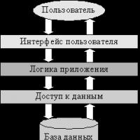 Distributed System Architecture Large Scale Cloud IoT Platform